15.3 Using DLMs to estimate changing season

Here is a DLM model with the level and season modeled as a random walk.

\[\begin{bmatrix}x \\ \beta_1 \\ \beta_2 \end{bmatrix}_t = \begin{bmatrix}x \\ \beta_1 \\ \beta_2 \end{bmatrix}_{t-1} + \begin{bmatrix}w_1 \\ w_2 \\ w_3 \end{bmatrix}_t\] \[y_t = \begin{bmatrix}1& \sin(2\pi t/p)&\cos(2\pi t/p)\end{bmatrix} \begin{bmatrix}x \\ \beta_1 \\ \beta_2 \end{bmatrix}_t + v_t\]

We can fit the model to the \(y_t\) data and estimate the \(\beta\)’s and \(\alpha\). We specify this one-to-one in R for MARSS().

Z is time-varying and we set this up with an array with the 3rd dimension being time.

Z <- array(1, dim = c(1, 3, TT))
Z[1, 2, ] <- sin(2 * pi * (1:TT)/12)
Z[1, 3, ] <- cos(2 * pi * (1:TT)/12)

Then we make our model list. We need to set A since MARSS() doesn’t like the default value of scaling when Z is time-varying.

mod.list <- list(U = "zero", Q = "diagonal and unequal", Z = Z, 
    A = "zero")

When we fit the model we need to give MARSS() initial values for x0. It cannot come up with default ones for this model. It doesn’t really matter what you pick.

require(MARSS)
fit <- MARSS(yt, model = mod.list, inits = list(x0 = matrix(0, 
    3, 1)))

Success! abstol and log-log tests passed at 45 iterations.
Alert: conv.test.slope.tol is 0.5.
Test with smaller values (<0.1) to ensure convergence.

MARSS fit is
Estimation method: kem 
Convergence test: conv.test.slope.tol = 0.5, abstol = 0.001
Estimation converged in 45 iterations. 
Log-likelihood: 19.0091 
AIC: -24.01821   AICc: -22.80082   
 
          Estimate
R.R        0.00469
Q.(X1,X1)  0.01476
Q.(X2,X2)  0.00638
Q.(X3,X3)  0.00580
x0.X1     -0.11002
x0.X2     -0.85340
x0.X3      0.92787
Initial states (x0) defined at t=0

Standard errors have not been calculated. 
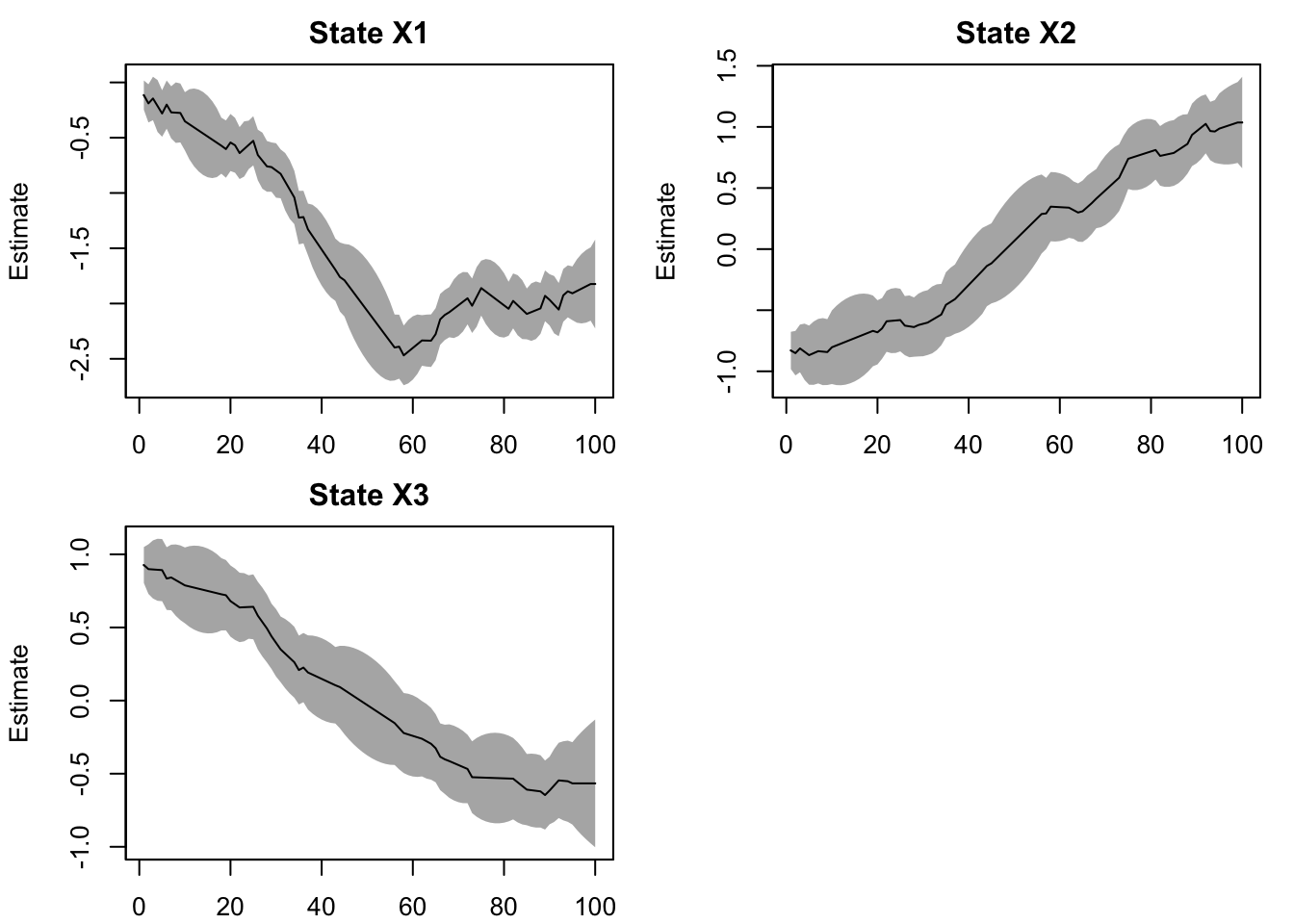
Use MARSSparamCIs to compute CIs and bias estimates.

The \(\beta_1\) estimate is State X2 and \(\beta_2\) is State X3. The estimates match what we put into the simulated data.

plot type = "xtT" Estimated states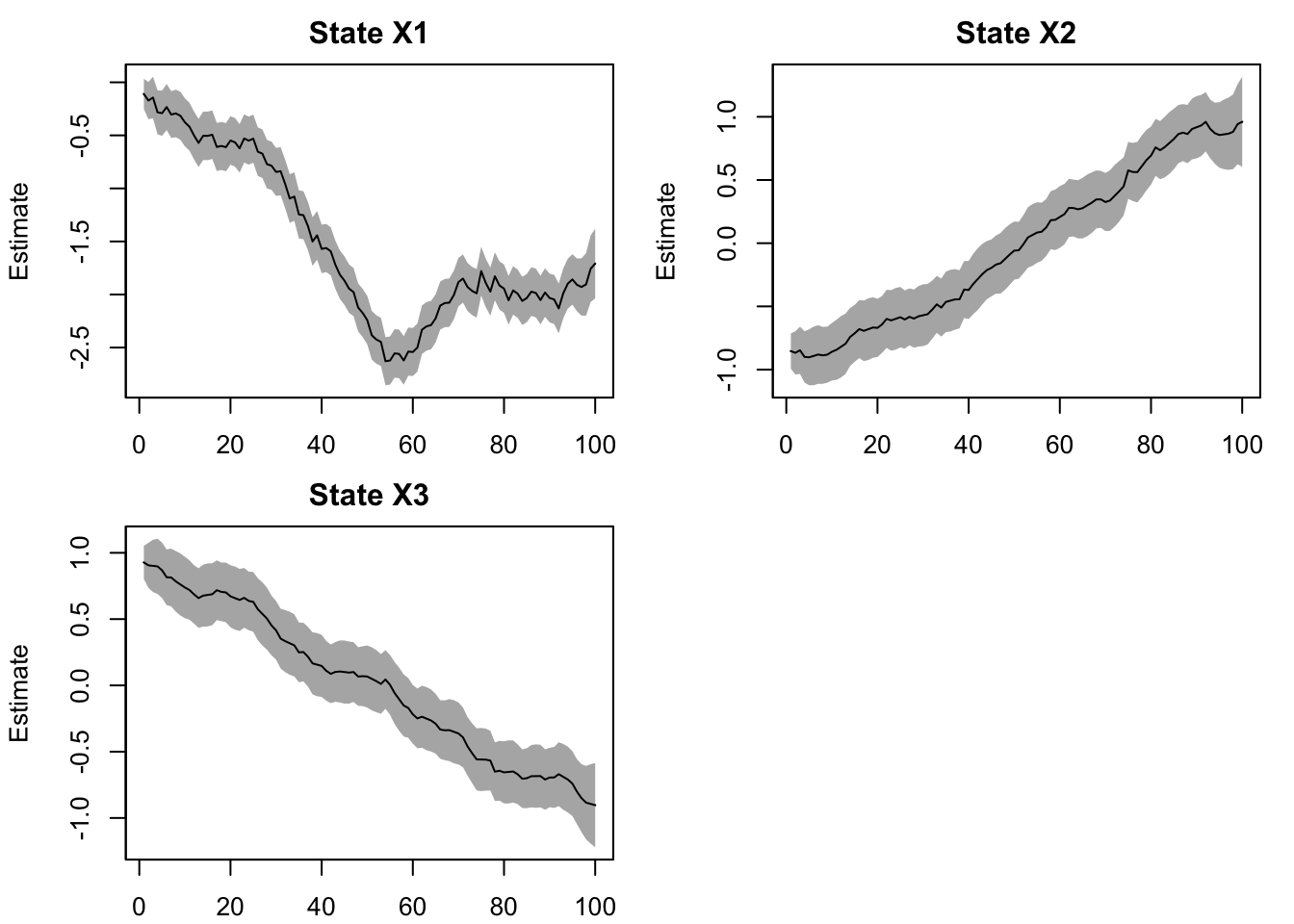

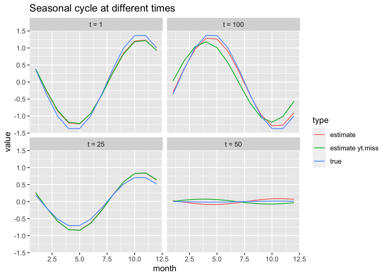
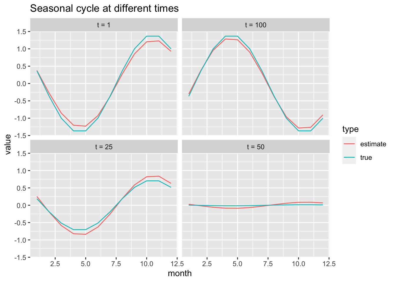
We can compare the estimated cycles to the ones used in the simulation.

We can make this a bit harder by imagining that our data have missing values. Let’s imagine that we only observe half the months.

yt.miss <- yt
yt.miss[sample(100, 50)] <- NA
plot(yt, type = "l")
points(yt.miss)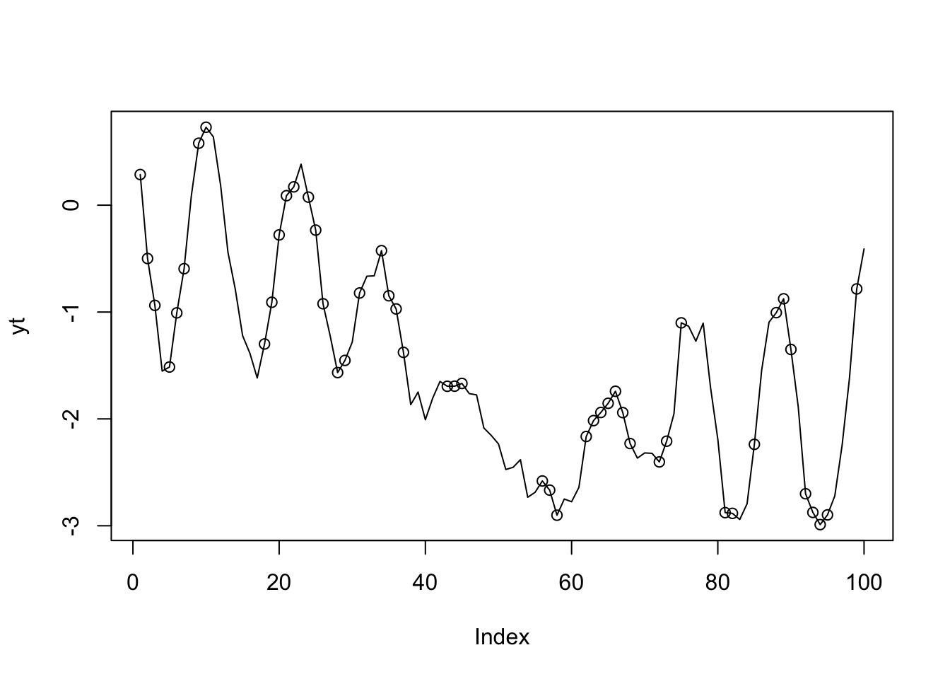

require(MARSS)
fit.miss <- MARSS(yt.miss, model = mod.list, inits = list(x0 = matrix(0, 
    3, 1)))

Success! abstol and log-log tests passed at 108 iterations.
Alert: conv.test.slope.tol is 0.5.
Test with smaller values (<0.1) to ensure convergence.

MARSS fit is
Estimation method: kem 
Convergence test: conv.test.slope.tol = 0.5, abstol = 0.001
Estimation converged in 108 iterations. 
Log-likelihood: 0.1948933 
AIC: 13.61021   AICc: 16.27688   
 
          Estimate
R.R        0.00243
Q.(X1,X1)  0.01342
Q.(X2,X2)  0.00794
Q.(X3,X3)  0.00580
x0.X1     -0.11497
x0.X2     -0.82921
x0.X3      0.92696
Initial states (x0) defined at t=0

Standard errors have not been calculated. 
Use MARSSparamCIs to compute CIs and bias estimates.

The model still can pick out the changing seasonal cycle.

plot type = "xtT" Estimated states