11.2 Example: Snotel Data
Let’s see an example using the Washington SNOTEL data. The data we will use is the snow water equivalent percent of normal. This represents the snow water equivalent compared to the average value for that site on the same day. We will look at a subset of sites in the Central Cascades in our snotel dataset (Figure 11.1).
y <- snotelmeta
# Just use a subset
y = y[which(y$Longitude < -121.4), ]
y = y[which(y$Longitude > -122.5), ]
y = y[which(y$Latitude < 47.5), ]
y = y[which(y$Latitude > 46.5), ]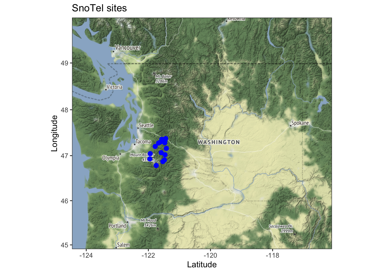
Figure 11.1: Subset of SNOTEL sties used in this chapter.
For the first analysis, we are just going to look at February Snow Water Equivalent (SWE). Our subset of stations is y$Station.Id. There are many missing years among some of our stations (Figure 11.2).
swe.feb <- snotel
swe.feb <- swe.feb[swe.feb$Station.Id %in% y$Station.Id & swe.feb$Month ==
    "Feb", ]
p <- ggplot(swe.feb, aes(x = Date, y = SWE)) + geom_line()
p + facet_wrap(~Station)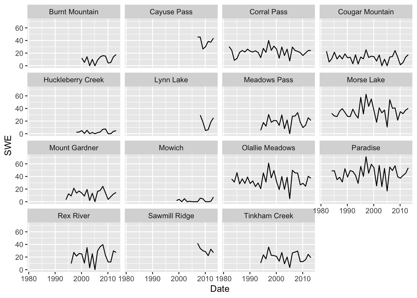
Figure 11.2: Snow water equivalent time series from each SNOTEL station.
11.2.1 Estimate missing Feb SWE using AR(1) with spatial correlation
Imagine that for our study we need an estimate of SWE for all sites. We will use the information from the sites with full data to estimate the missing SWE for other sites. We will use a MARSS model to use all the available data.
\[\begin{equation} \begin{gathered} \begin{bmatrix} x_1 \\ x_2 \\ \dots \\ x_{15} \end{bmatrix}_t = \begin{bmatrix} b&0&\dots&0 \\ 0&b&\dots&0 \\ \dots&\dots&\dots&\dots \\ 0&0&\dots&b \end{bmatrix} \begin{bmatrix} x_1 \\ x_2 \\ \dots \\ x_{15} \end{bmatrix}_{t-1} + \begin{bmatrix} w_1 \\ w_2 \\ \dots \\ w_{15} \end{bmatrix}_{t} \\ \begin{bmatrix} y_1 \\ y_2 \\ \dots \\ y_{15} \end{bmatrix}_t = \begin{bmatrix} x_1 \\ x_2 \\ \dots \\ x_{15} \end{bmatrix}_t + \begin{bmatrix} a_1 \\ a_2 \\ \dots \\ a_{15} \end{bmatrix}_{t} + \begin{bmatrix} v_1 \\ v_2 \\ \dots \\ v_{15} \end{bmatrix}_t \end{gathered} \tag{11.5} \end{equation}\]
We will use an unconstrained variance-covariance structure for \(\mathbf{w}\) and assume that \(\mathbf{v}\) is identical and independent and very low (SNOTEL instrument variability). The \(a_i\) determine the level of the \(x_i\).
We need our data to be in rows. We will use reshape2::acast().
dat.feb <- reshape2::acast(swe.feb, Station ~ Year, value.var = "SWE")We set up the model for MARSS so that it is the same as (11.5). We will fix the measurement error to be small; we could use 0 but the fitting is more stable if we use a small variance instead. When estimating \(\mathbf{B}\), setting the initial value to be at \(t=1\) instead of \(t=0\) works better.
ns <- length(unique(swe.feb$Station))
B <- "diagonal and equal"
Q <- "unconstrained"
R <- diag(0.01, ns)
U <- "zero"
A <- "unequal"
x0 <- "unequal"
mod.list.ar1 = list(B = B, Q = Q, R = R, U = U, x0 = x0, A = A,
    tinitx = 1)
Now we can fit a MARSS model and get estimates of the missing SWEs. Convergence is slow. We set \(\mathbf{a}\) equal to the mean of the time series to speed convergence.
library(MARSS)
m <- apply(dat.feb, 1, mean, na.rm = TRUE)
fit.ar1 <- MARSS(dat.feb, model = mod.list.ar1, control = list(maxit = 5000),
    inits = list(A = matrix(m, ns, 1)))
The \(b\) estimate is 0.4494841.
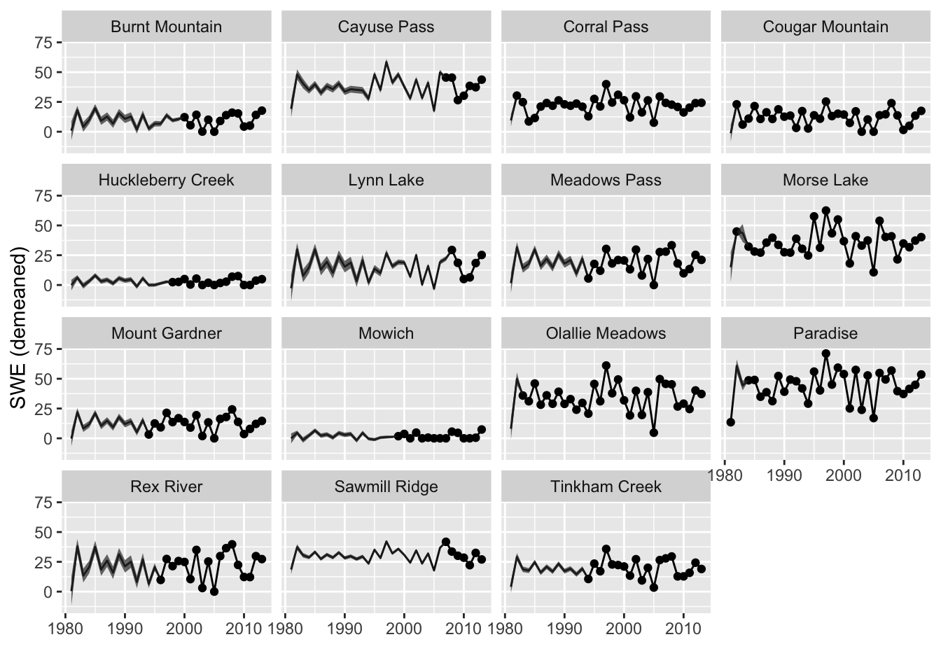
Let’s plot the estimated SWEs for the missing years (Figure 11.3). These estimates use all the information about the correlation with other sites and uses information about correlation with the prior and subsequent years. We will use the tidy() function to get the estimates and the 95% prediction intervals. The prediction interval is for the range of SWE values we might observe for that site. Notice that for some sites, intervals are low in early years as these sites are highly correlated with site for which there are data. In other sites, the uncertainty is high in early years because the sites with data in those years are not highly correlated. There are no intervals for sites with data. We have data for those sites, so we are not uncertain about the observed SWE for those.
fit <- fit.ar1
d <- fitted(fit, interval = "prediction", type = "ytT")
d$Year <- d$t + 1980
d$Station <- d$.rownames
p <- ggplot(data = d) + geom_line(aes(Year, .fitted)) + geom_point(aes(Year,
    y)) + geom_ribbon(aes(x = Year, ymin = .lwr, ymax = .upr),
    linetype = 2, alpha = 0.2, fill = "blue") + facet_wrap(~Station) +
    xlab("") + ylab("SWE (demeaned)")
p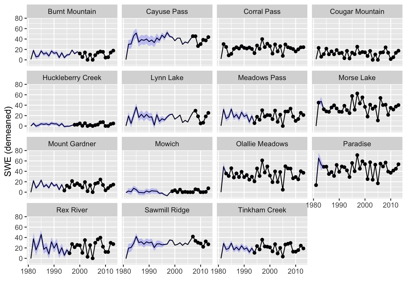
Figure 11.3: Estimated SWEs for the missing sites with prediction intervals.
If we were using these SWE as covariates in a site specific model, we could then use the estimates as our covariates, however this would not incorporate parameter uncertainty. Alternatively we could use Equation (11.1) and set the parameters for the covariate process to those estimated for our covariate-only model. This approach will incorporate the uncertainty in the SWE estimates in the early years for the sites with no data.
Note, we should do some cross-validation (fitting with data left out) to ensure that the estimated SWEs are well-matched to actual measurements. It would probably be best to do ‘leave-three’ out instead of ‘leave-one’ out since the estimates for time \(t\) uses information from \(t-1\) and \(t+1\) (if present).
11.2.1.1 Diagnostics
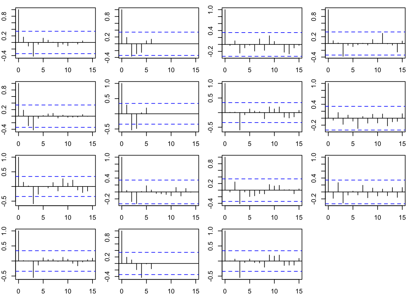
The model residuals have a tendency for negative autocorrelation at lag-1 (Figure 11.4).
fit <- fit.ar1
par(mfrow = c(4, 4), mar = c(2, 2, 1, 1))
apply(MARSSresiduals(fit, type = "tt1")$model.residuals[, 1:30],
    1, acf, na.action = na.pass)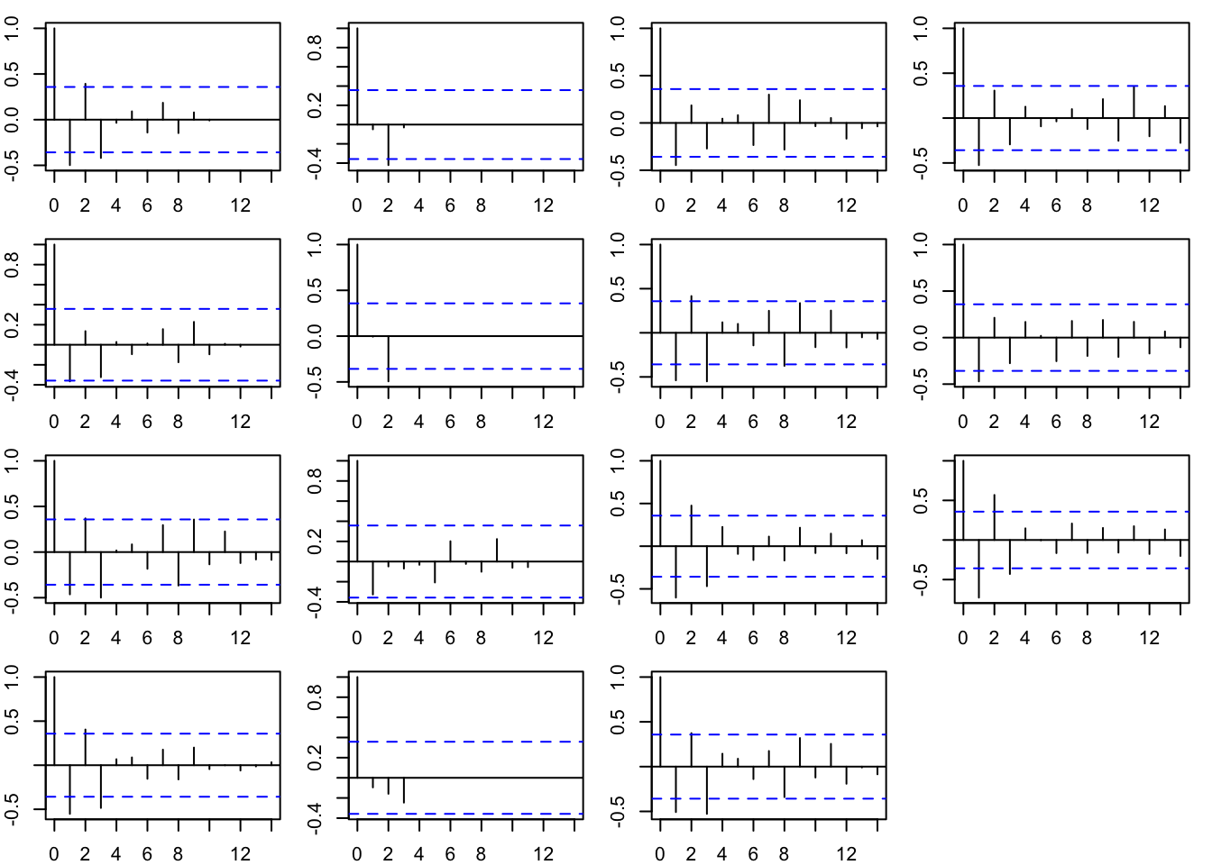
Figure 11.4: Model residuals for the AR(1) model.
11.2.2 Estimate missing Feb SWE using only correlation
Another approach is to treat the February data as temporally uncorrelated. The two longest time series (Paradise and Olallie Meadows) show minimal autocorrelation so we might decide to just use the correlation across stations for our estimates. In this case, the state of the missing SWE values at time \(t\) is the expected value conditioned on all the stations with data at time \(t\) given the estimated variance-covariance matrix \(\mathbf{Q}\).
We could set this model up as \[\begin{equation} \begin{bmatrix} y_1 \\ y_2 \\ \dots \\ y_{15} \end{bmatrix}_t = \begin{bmatrix} a_1 \\ a_2 \\ \dots \\ a_{15} \end{bmatrix}_{t} + \begin{bmatrix} v_1 \\ v_2 \\ \dots \\ v_{15} \end{bmatrix}_t, \,\,\, \begin{bmatrix} \sigma_1&\zeta_{1,2}&\dots&\zeta_{1,15} \\ \zeta_{2,1}&\sigma_2&\dots&\zeta_{2,15} \\ \dots&\dots&\dots&\dots \\ \zeta_{15,1}&\zeta_{15,2}&\dots&\sigma_{15} \end{bmatrix} \tag{11.6} \end{equation}\]
However the EM algorithm used by MARSS() runs into numerical issues. Instead we will set the model up as follows. Allowing a hidden state observed with small error makes the estimation more stable.
\[\begin{equation} \begin{gathered} \begin{bmatrix} x_1 \\ x_2 \\ \dots \\ x_{15} \end{bmatrix}_t = \begin{bmatrix} w_1 \\ w_2 \\ \dots \\ w_{15} \end{bmatrix}_{t}, \,\,\, \begin{bmatrix} w_1 \\ w_2 \\ \dots \\ w_{15} \end{bmatrix}_{t} \sim \begin{bmatrix} \sigma_1&\zeta_{1,2}&\dots&\zeta_{1,15} \\ \zeta_{2,1}&\sigma_2&\dots&\zeta_{2,15} \\ \dots&\dots&\dots&\dots \\ \zeta_{15,1}&\zeta_{15,2}&\dots&\sigma_{15} \end{bmatrix} \\ \begin{bmatrix} y_1 \\ y_2 \\ \dots \\ y_{15} \end{bmatrix}_t = \begin{bmatrix} x_1 \\ x_2 \\ \dots \\ x_{15} \end{bmatrix}_t + \begin{bmatrix} a_1 \\ a_2 \\ \dots \\ a_{15} \end{bmatrix}_{t} + \begin{bmatrix} v_1 \\ v_2 \\ \dots \\ v_{15} \end{bmatrix}_t, \,\,\, \begin{bmatrix} 0.01&0&\dots&0 \\ 0&0.01&\dots&0 \\ \dots&\dots&\dots&\dots \\ 0&0&\dots&0.01 \end{bmatrix} \end{gathered} \tag{11.7} \end{equation}\] Again \(\mathbf{a}\) is the mean level in the time series. Note that the expected value of \(\mathbf{x}\) is zero if there are no data, so \(E(\mathbf{x}_0)=0\).
ns <- length(unique(swe.feb$Station))
B <- "zero"
Q <- "unconstrained"
R <- diag(0.01, ns)
U <- "zero"
A <- "unequal"
x0 <- "zero"
mod.list.corr = list(B = B, Q = Q, R = R, U = U, x0 = x0, A = A,
    tinitx = 0)
Now we can fit a MARSS model and get estimates of the missing SWEs. Convergence is slow. We set \(\mathbf{a}\) equal to the mean of the time series to speed convergence.
m <- apply(dat.feb, 1, mean, na.rm = TRUE)
fit.corr <- MARSS(dat.feb, model = mod.list.corr, control = list(maxit = 5000),
    inits = list(A = matrix(m, ns, 1)))
The estimated SWEs for the missing years uses the information about the correlation with other sites only.
fit <- fit.corr
d <- fitted(fit, type = "ytT", interval = "prediction")
d$Year <- d$t + 1980
d$Station <- d$.rownames
p <- ggplot(data = d) + geom_line(aes(Year, .fitted)) + geom_point(aes(Year,
    y)) + geom_ribbon(aes(x = Year, ymin = .lwr, ymax = .upr),
    linetype = 2, alpha = 0.2, fill = "blue") + facet_wrap(~Station) +
    xlab("") + ylab("SWE (demeaned)")
p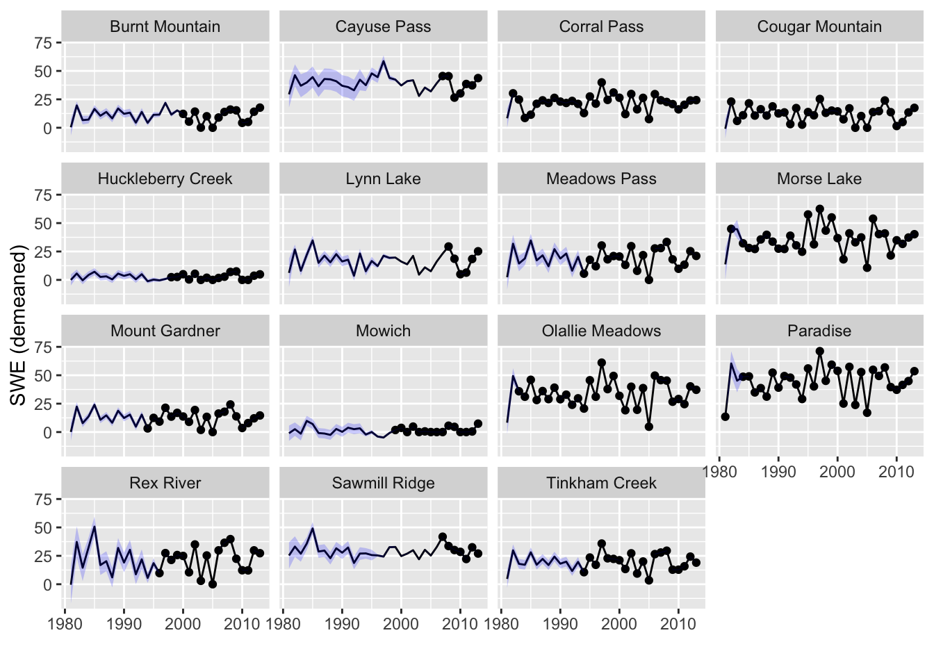
Figure 11.5: Estimated SWEs from the expected value of the states \(\hat{x}\) conditioned on all the data for the model with only correlation across stations at time \(t\).
11.2.2.1 Diagnostics
The model residuals have no tendency towards negative autocorrelation now that we removed the autoregressive component from the process (\(x\)) model.
fit <- fit.corr
par(mfrow = c(4, 4), mar = c(2, 2, 1, 1))
apply(MARSSresiduals(fit, type = "tt1")$model.residuals, 1, acf,
    na.action = na.pass)
mtext("Model Residuals ACF", outer = TRUE, side = 3)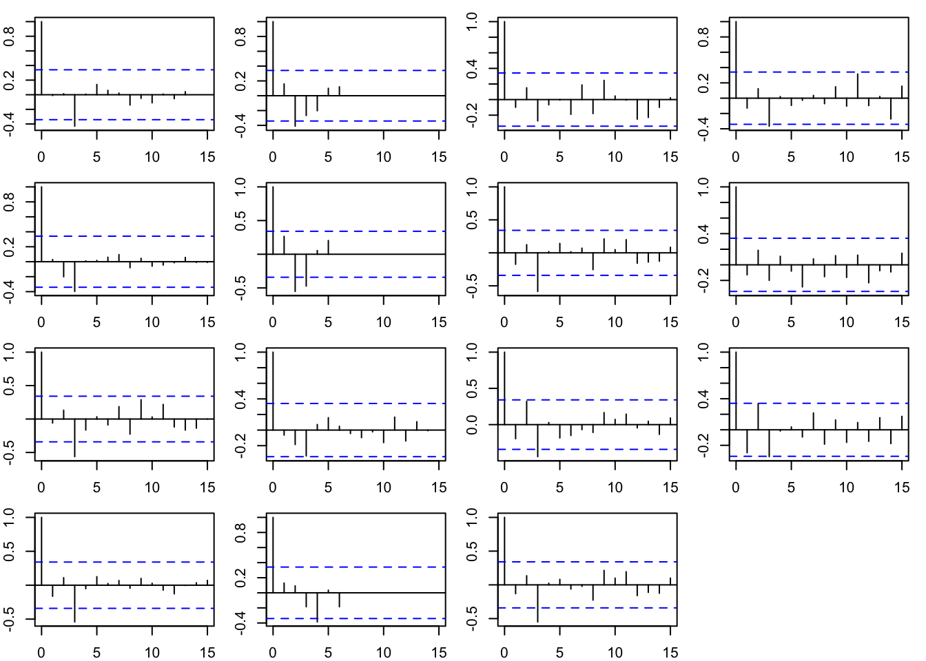
11.2.3 Estimate missing Feb SWE using DFA
Another approach we might take is to model SWE using Dynamic Factor Analysis. Our model might take the following form with two factors, modeled as AR(1) processes. \(\mathbf{a}\) is the mean level of the time series.
\[\begin{equation} \begin{gathered} \begin{bmatrix} x_1 \\ x_2 \end{bmatrix}_t = \begin{bmatrix} b_1&0\\0&b_2 \end{bmatrix} \begin{bmatrix} x_1 \\ x_2 \end{bmatrix}_{t-1} + \begin{bmatrix} w_1 \\ w_2 \end{bmatrix}_{t} \\ \begin{bmatrix} y_1 \\ y_2 \\ \dots \\ y_{15} \end{bmatrix}_t = \begin{bmatrix} z_{1,1}&0\\z_{2,1}&z_{2,2}\\ \dots\\z_{3,1}&z_{3,2} \end{bmatrix}\begin{bmatrix} x_1 \\ x_2 \end{bmatrix}_t + \begin{bmatrix} a_1 \\ a_2 \\ \dots \\ a_{15} \end{bmatrix} + \begin{bmatrix} v_1 \\ v_2 \\ \dots \\ v_{15} \end{bmatrix}_t \end{gathered} \end{equation}\]
The model is set up as follows:
ns <- dim(dat.feb)[1]
B <- matrix(list(0), 2, 2)
B[1, 1] <- "b1"
B[2, 2] <- "b2"
Q <- diag(1, 2)
R <- "diagonal and unequal"
U <- "zero"
x0 <- "zero"
Z <- matrix(list(0), ns, 2)
Z[1:(ns * 2)] <- c(paste0("z1", 1:ns), paste0("z2", 1:ns))
Z[1, 2] <- 0
A <- "unequal"
mod.list.dfa = list(B = B, Z = Z, Q = Q, R = R, U = U, A = A,
    x0 = x0)
Now we can fit a MARSS model and get estimates of the missing SWEs. We pass in the initial value for \(\mathbf{a}\) as the mean level so it fits easier.
library(MARSS)
m <- apply(dat.feb, 1, mean, na.rm = TRUE)
fit.dfa <- MARSS(dat.feb, model = mod.list.dfa, control = list(maxit = 1000),
    inits = list(A = matrix(m, ns, 1)))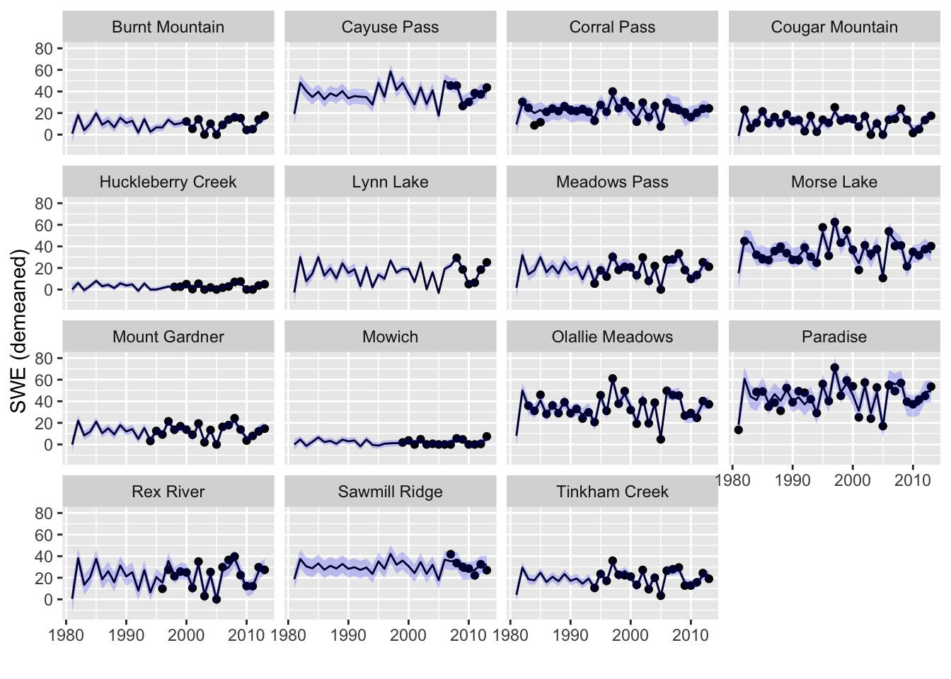
11.2.4 Diagnostics
The model residuals are uncorrelated.
par(mfrow = c(4, 4), mar = c(2, 2, 1, 1))
apply(MARSSresiduals(fit, type = "tt1")$model.residual, 1, function(x) {
    acf(x, na.action = na.pass)
})
11.2.5 Plot the fitted or mean Feb SWE using DFA
The plots showed the estimate of the missing Feb SWE values, which is the expected value of \(\mathbf{y}\) conditioned on all the data. For the non-missing SWE, this expected value is just the observation. Many times we want the model fit for the covariate. If the measurements have observation error, the fitted value is the estimate without this observation error.
For the estimated states conditioned on all the data we want tsSmooth(). We will not show the prediction intervals which would be for new data. We will just show the confidence intervals on the fitted estimate for the missing values. The confidence intervals are small so they are a bit hard to see.