16.4 Univariate results

Plot of the amplitude of the cycles. All the rivers were analyzed independently. It certainly looks like there are common patterns in the amplitude of the cycles with many showing a steady decline in amplitude. Note the counts were not decreasing so this is not due to fewer spawners.

ggplot(dfz, aes(x = brood_year, y = amplitude)) + geom_line() + 
    facet_wrap(~river, scales = "free_y") + ggtitle("Cycle Amplitude")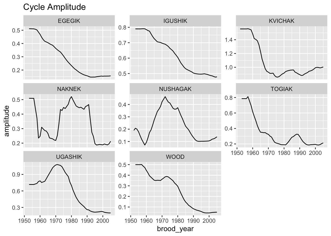

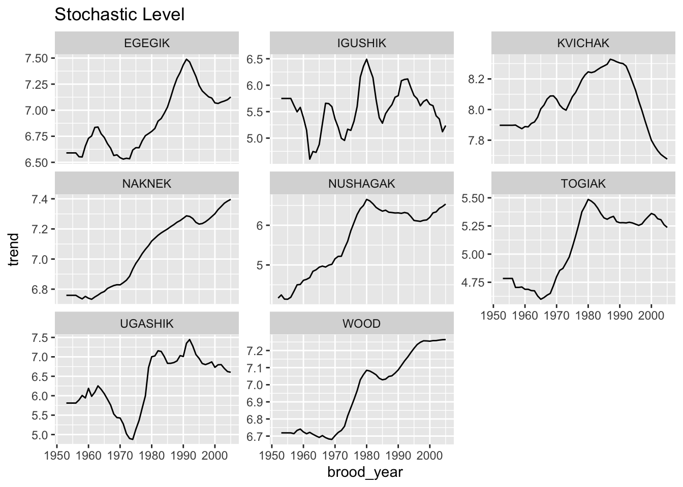
Plot of the stochastic level. Again all the rivers were analyzed independently. It certainly looks like there are common patterns in the trends. In the next step, we can test this.

ggplot(dfz, aes(x = brood_year, y = trend)) + geom_line() + facet_wrap(~river, 
    scales = "free_y") + ggtitle("Stochastic Level")