10.9 Estimated states and loadings

Here are plots of the three hidden processes (left column) and the loadings for each of phytoplankton groups (right column).

ylbl <- phytoplankton
w_ts <- seq(dim(dat)[2])
layout(matrix(c(1, 2, 3, 4, 5, 6), mm, 2), widths = c(2, 1))
## par(mfcol=c(mm,2), mai = c(0.5,0.5,0.5,0.1), omi =
## c(0,0,0,0))
par(mai = c(0.5, 0.5, 0.5, 0.1), omi = c(0, 0, 0, 0))
## plot the processes
for (i in 1:mm) {
    ylm <- c(-1, 1) * max(abs(proc_rot[i, ]))
    ## set up plot area
    plot(w_ts, proc_rot[i, ], type = "n", bty = "L", ylim = ylm, 
        xlab = "", ylab = "", xaxt = "n")
    ## draw zero-line
    abline(h = 0, col = "gray")
    ## plot trend line
    lines(w_ts, proc_rot[i, ], lwd = 2)
    lines(w_ts, proc_rot[i, ], lwd = 2)
    ## add panel labels
    mtext(paste("State", i), side = 3, line = 0.5)
    axis(1, 12 * (0:dim(dat_1980)[2]) + 1, yr_frst + 0:dim(dat_1980)[2])
}
## plot the loadings
minZ <- 0
ylm <- c(-1, 1) * max(abs(Z_rot))
for (i in 1:mm) {
    plot(c(1:N_ts)[abs(Z_rot[, i]) > minZ], as.vector(Z_rot[abs(Z_rot[, 
        i]) > minZ, i]), type = "h", lwd = 2, xlab = "", ylab = "", 
        xaxt = "n", ylim = ylm, xlim = c(0.5, N_ts + 0.5), col = clr)
    for (j in 1:N_ts) {
        if (Z_rot[j, i] > minZ) {
            text(j, -0.03, ylbl[j], srt = 90, adj = 1, cex = 1.2, 
                col = clr[j])
        }
        if (Z_rot[j, i] < -minZ) {
            text(j, 0.03, ylbl[j], srt = 90, adj = 0, cex = 1.2, 
                col = clr[j])
        }
        abline(h = 0, lwd = 1.5, col = "gray")
    }
    mtext(paste("Factor loadings on state", i), side = 3, line = 0.5)
}

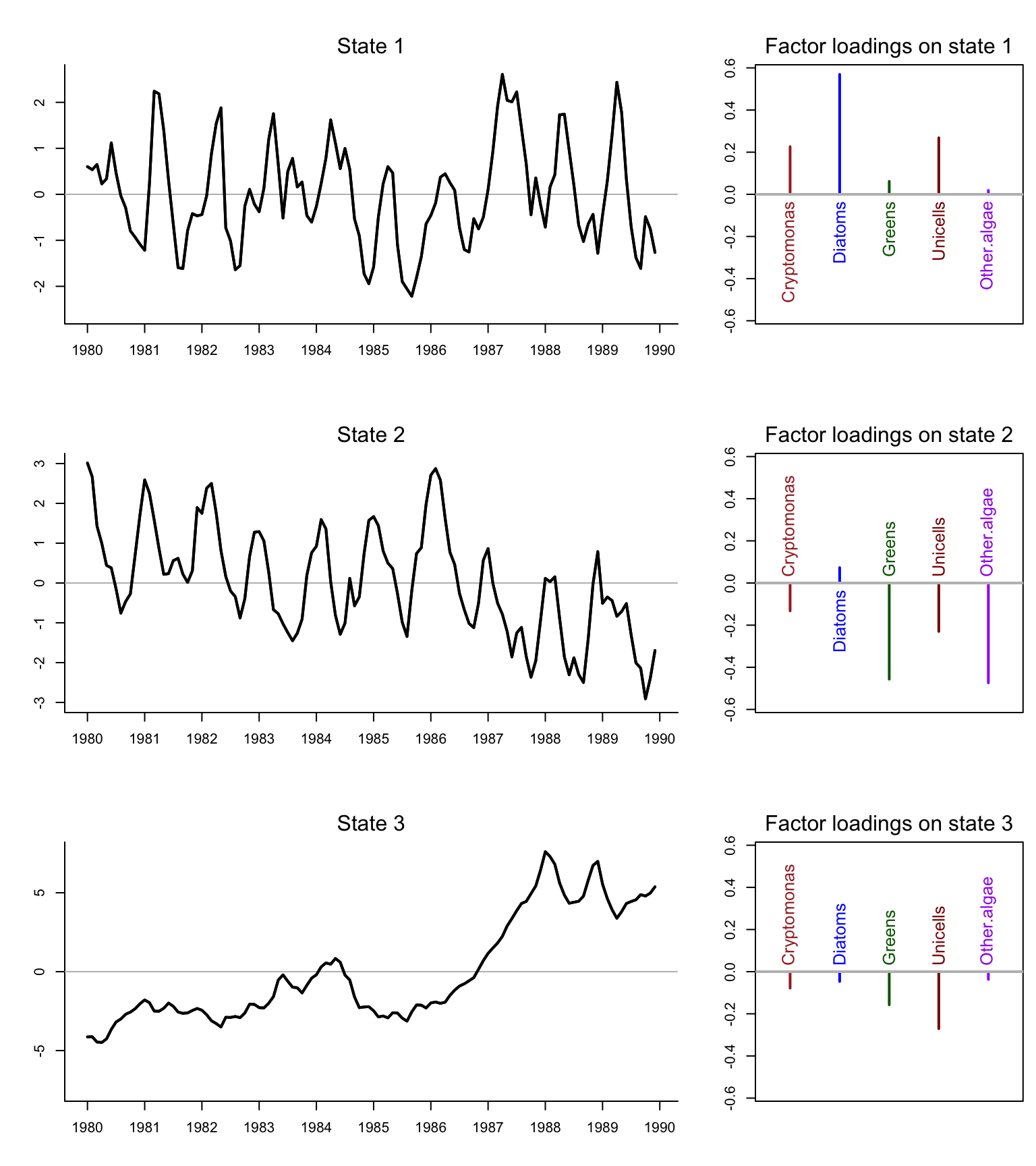
Figure 10.2: Estimated states from the DFA model.

It looks like there are strong seasonal cycles in the data, but there is some indication of a phase difference between some of the groups. We can use ccf() to investigate further.

par(mai = c(0.9, 0.9, 0.1, 0.1))
ccf(proc_rot[1, ], proc_rot[2, ], lag.max = 12, main = "")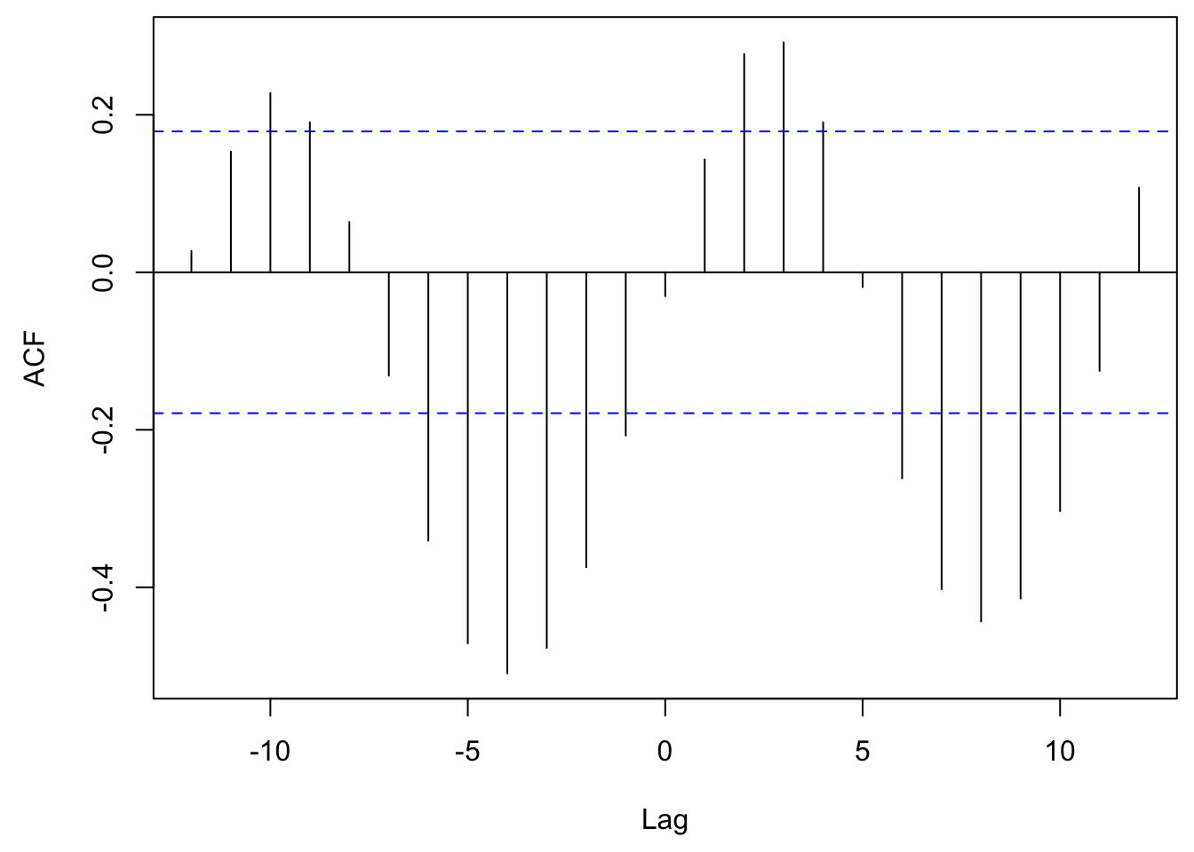

Figure 10.3: Cross-correlation plot of the two rotations.