4.2 Decomposition of time series

Plotting time series data is an important first step in analyzing their various components. Beyond that, however, we need a more formal means for identifying and removing characteristics such as a trend or seasonal variation. As discussed in lecture, the decomposition model reduces a time series into 3 components: trend, seasonal effects, and random errors. In turn, we aim to model the random errors as some form of stationary process.

Let’s begin with a simple, additive decomposition model for a time series $x_t$

\[\begin{equation} \tag{4.1} x_t = m_t + s_t + e_t, \end{equation}\]

where, at time $t$, $m_t$ is the trend, $s_t$ is the seasonal effect, and $e_t$ is a random error that we generally assume to have zero-mean and to be correlated over time. Thus, by estimating and subtracting both $\{m_t\}$ and $\{s_t\}$ from $\{x_t\}$, we hope to have a time series of stationary residuals $\{e_t\}$.

4.2.1 Estimating trends

In lecture we discussed how linear filters are a common way to estimate trends in time series. One of the most common linear filters is the moving average, which for time lags from $-a$ to $a$ is defined as

\[\begin{equation} \tag{4.2} \hat{m}_t = \sum_{k=-a}^{a} \left(\frac{1}{1+2a}\right) x_{t+k}. \end{equation}\]

This model works well for moving windows of odd-numbered lengths, but should be adjusted for even-numbered lengths by adding only $\frac{1}{2}$ of the 2 most extreme lags so that the filtered value at time $t$ lines up with the original observation at time $t$. So, for example, in a case with monthly data such as the atmospheric CO$_2$ concentration where a 12-point moving average would be an obvious choice, the linear filter would be

\[\begin{equation} \tag{4.3} \hat{m}_t = \frac{\frac{1}{2}x_{t-6} + x_{t-5} + \dots + x_{t-1} + x_t + x_{t+1} + \dots + x_{t+5} + \frac{1}{2}x_{t+6}}{12} \end{equation}\]

It is important to note here that our time series of the estimated trend $\{\hat{m}_t\}$ is actually shorter than the observed time series by $2a$ units.

Conveniently, R has the built-in function filter() in the stats package for estimating moving-average (and other) linear filters. In addition to specifying the time series to be filtered, we need to pass in the filter weights (and 2 other arguments we won’t worry about here–type ?filter to get more information). The easiest way to create the filter is with the rep() function:

## weights for moving avg
fltr <- c(1/2, rep(1, times = 11), 1/2)/12

Now let’s get our estimate of the trend $\{\hat{m}\}$ with filter()} and plot it:

## estimate of trend
co2_trend <- stats::filter(co2, filter = fltr, method = "convo", 
    sides = 2)
## plot the trend
plot.ts(co2_trend, ylab = "Trend", cex = 1)

The trend is a more-or-less smoothly increasing function over time, the average slope of which does indeed appear to be increasing over time as well (Figure 4.3).

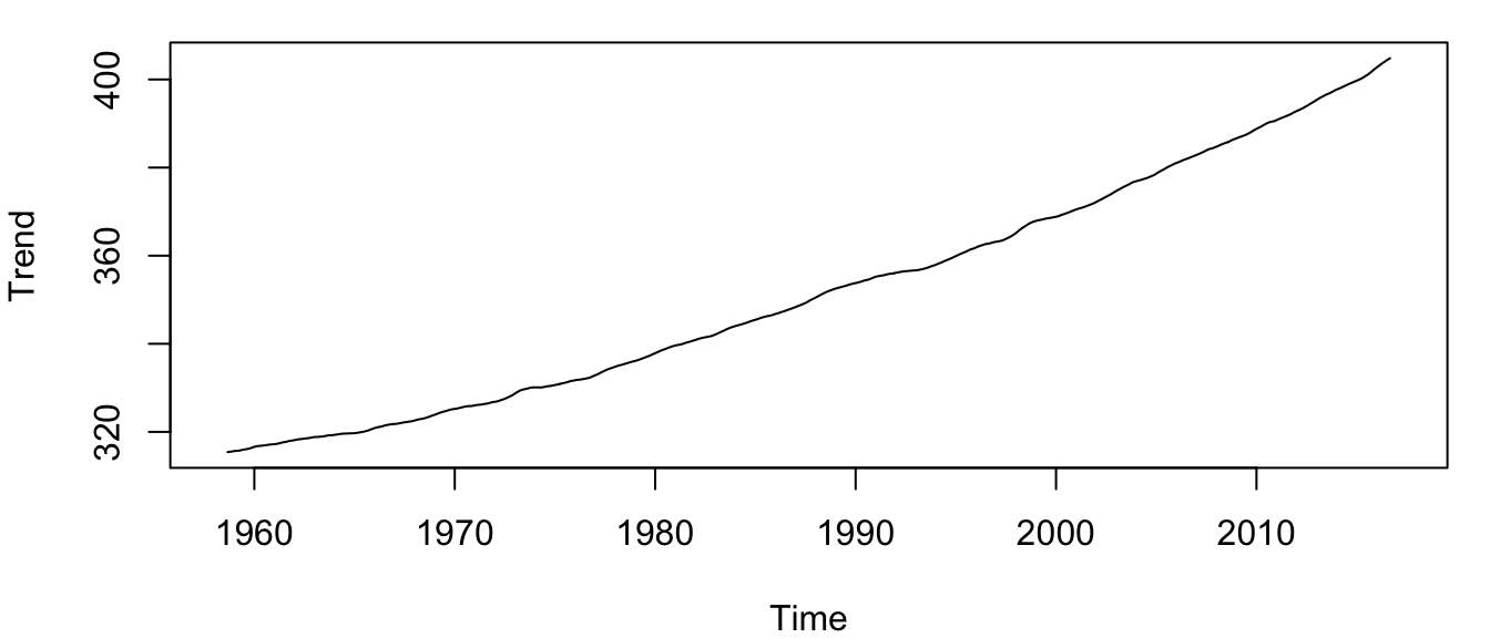
$Time series of the estimated trend $\{\hat{m}_t\}$ for the atmospheric CO$_2$ concentration at Mauna Loa, Hawai’i.$

Figure 4.3: Time series of the estimated trend $\{\hat{m}_t\}$ for the atmospheric CO$_2$ concentration at Mauna Loa, Hawai’i.

4.2.2 Estimating seasonal effects

Once we have an estimate of the trend for time $t$ ($\hat{m}_t$) we can easily obtain an estimate of the seasonal effect at time $t$ ($\hat{s}_t$) by subtraction

\[\begin{equation} \tag{4.4} \hat{s}_t = x_t - \hat{m}_t, \end{equation}\]

which is really easy to do in R:

## seasonal effect over time
co2_seas <- co2 - co2_trend

This estimate of the seasonal effect for each time $t$ also contains the random error $e_t$, however, which can be seen by plotting the time series and careful comparison of Equations (4.1) and (4.4).

## plot the monthly seasonal effects
plot.ts(co2_seas, ylab = "Seasonal effect", xlab = "Month", cex = 1)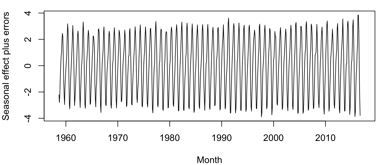

$Time series of seasonal effects plus random errors for the atmospheric CO$_2$ concentration at Mauna Loa, Hawai’i, measured monthly from March 1958 to present.$

Figure 4.4: Time series of seasonal effects plus random errors for the atmospheric CO$_2$ concentration at Mauna Loa, Hawai’i, measured monthly from March 1958 to present.

We can obtain the overall seasonal effect by averaging the estimates of $\{\hat{s}_t\}$ for each month and repeating this sequence over all years.

## length of ts
ll <- length(co2_seas)
## frequency (ie, 12)
ff <- frequency(co2_seas)
## number of periods (years); %/% is integer division
periods <- ll%/%ff
## index of cumulative month
index <- seq(1, ll, by = ff) - 1
## get mean by month
mm <- numeric(ff)
for (i in 1:ff) {
    mm[i] <- mean(co2_seas[index + i], na.rm = TRUE)
}
## subtract mean to make overall mean = 0
mm <- mm - mean(mm)

Before we create the entire time series of seasonal effects, let’s plot them for each month to see what is happening within a year:

## plot the monthly seasonal effects
plot.ts(mm, ylab = "Seasonal effect", xlab = "Month", cex = 1)

It looks like, on average, that the CO$_2$ concentration is highest in spring (March) and lowest in summer (August) (Figure 4.5). (Aside: Do you know why this is?)

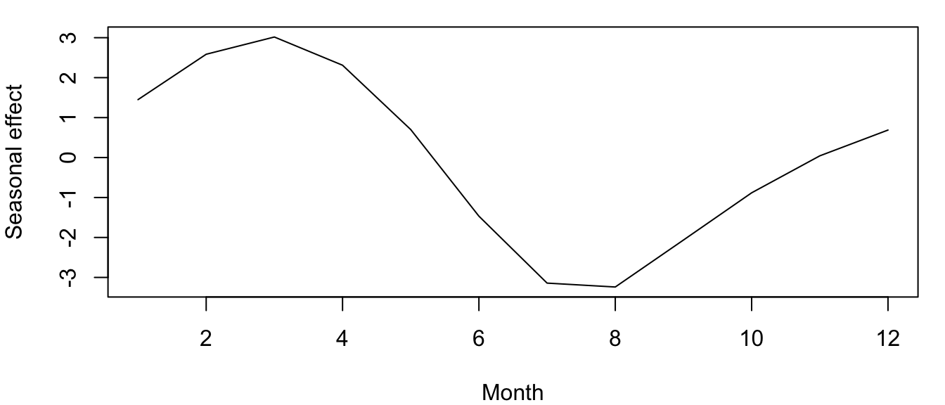
$Estimated monthly seasonal effects for the atmospheric CO$_2$ concentration at Mauna Loa, Hawai’i.$

Figure 4.5: Estimated monthly seasonal effects for the atmospheric CO$_2$ concentration at Mauna Loa, Hawai’i.

Finally, let’s create the entire time series of seasonal effects $\{\hat{s}_t\}$:

## create ts object for season
co2_seas_ts <- ts(rep(mm, periods + 1)[seq(ll)], start = start(co2_seas), 
    frequency = ff)

4.2.3 Completing the model

The last step in completing our full decomposition model is obtaining the random errors $\{\hat{e}_t\}$, which we can get via simple subtraction

\[\begin{equation} \tag{4.5} \hat{e}_t = x_t - \hat{m}_t - \hat{s}_t. \end{equation}\]

Again, this is really easy in R:

## random errors over time
co2_err <- co2 - co2_trend - co2_seas_ts

Now that we have all 3 of our model components, let’s plot them together with the observed data $\{x_t\}$. The results are shown in Figure 4.6.

## plot the obs ts, trend & seasonal effect
plot(cbind(co2, co2_trend, co2_seas_ts, co2_err), main = "", 
    yax.flip = TRUE)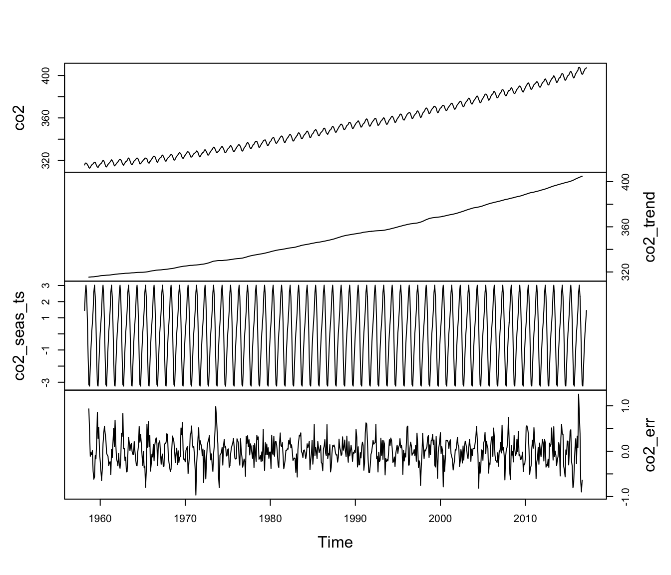

$Time series of the observed atmospheric CO$_2$ concentration at Mauna Loa, Hawai’i (top) along with the estimated trend, seasonal effects, and random errors.$

Figure 4.6: Time series of the observed atmospheric CO$_2$ concentration at Mauna Loa, Hawai’i (top) along with the estimated trend, seasonal effects, and random errors.

4.2.4 Using `decompose()` for decomposition

Now that we have seen how to estimate and plot the various components of a classical decomposition model in a piecewise manner, let’s see how to do this in one step in R with the function decompose(), which accepts a ts object as input and returns an object of class decomposed.ts.

## decomposition of CO2 data
co2_decomp <- decompose(co2)

co2_decomp is a list with the following elements, which should be familiar by now:

x: the observed time series $\{x_t\}$
seasonal: time series of estimated seasonal component $\{\hat{s}_t\}$
figure: mean seasonal effect (length(figure) == frequency(x))
trend: time series of estimated trend $\{\hat{m}_t\}$
random: time series of random errors $\{\hat{e}_t\}$
type: type of error ("additive" or "multiplicative")

We can easily make plots of the output and compare them to those in Figure 4.6:

## plot the obs ts, trend & seasonal effect
plot(co2_decomp, yax.flip = TRUE)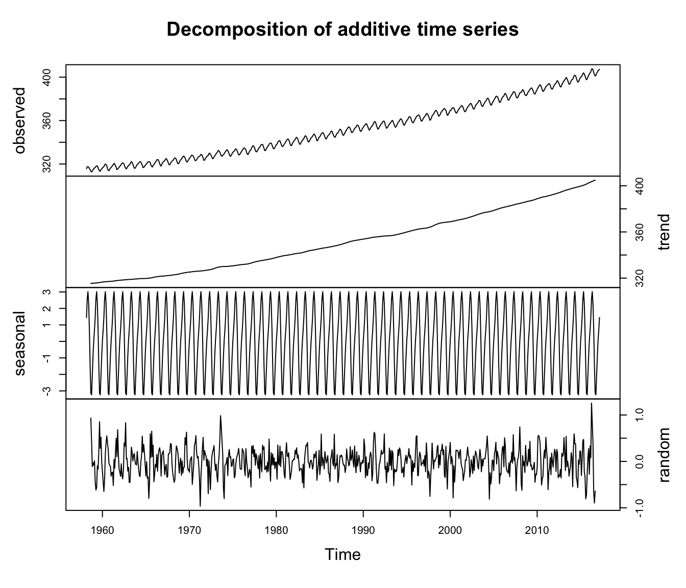

$Time series of the observed atmospheric CO$_2$ concentration at Mauna Loa, Hawai’i (top) along with the estimated trend, seasonal effects, and random errors obtained with the function decompose().$

Figure 4.7: Time series of the observed atmospheric CO$_2$ concentration at Mauna Loa, Hawai’i (top) along with the estimated trend, seasonal effects, and random errors obtained with the function decompose().

The results obtained with decompose() (Figure 4.7) are identical to those we estimated previously.

Another nice feature of the decompose() function is that it can be used for decomposition models with multiplicative (i.e., non-additive) errors (e.g., if the original time series had a seasonal amplitude that increased with time). To do, so pass in the argument type = "multiplicative", which is set to type = "additive" by default.