7.5 Four subpopulations with temporally correlated errors

Another reasonable assumption is that the different census regions are measuring different subpopulations but that the year-to-year population growth rates are correlated (good and bad year coincide). The only parameter that changes is the \(\mathbf{Q}\) matrix: \[\begin{equation} \mathbf{Q}=\begin{bmatrix} q & c & c & c \\ c & q & c & c\\ c & c & q & c \\ c & c & c & q \end{bmatrix} \tag{7.9} \end{equation}\] This \(\mathbf{Q}\) matrix structure means that the process variance (variance in year-to-year population growth rates) is the same across regions and the covariance in year-to-year population growth rates is also the same across regions.

7.5.1 Fitting the model

Set up the model list for MARSS() as:

mod.list.2 <- mod.list.1
mod.list.2$Q <- "equalvarcov"

"equalvarcov" is a shortcut for the matrix form in Equation (7.9).

Fit the model with:

fit.2 <- MARSS::MARSS(dat, model = mod.list.2)

Results are not shown, but here are the AICc. This last model is much better:

c(fit.0$AICc, fit.1$AICc, fit.2$AICc)

[1] -19.02786 -22.20194 -41.00511

7.5.2 Model residuals

Look at the model residuals (Figure 7.3). They are also much better.

MARSSresiduals.tt1 reported warnings. See msg element of returned residuals object.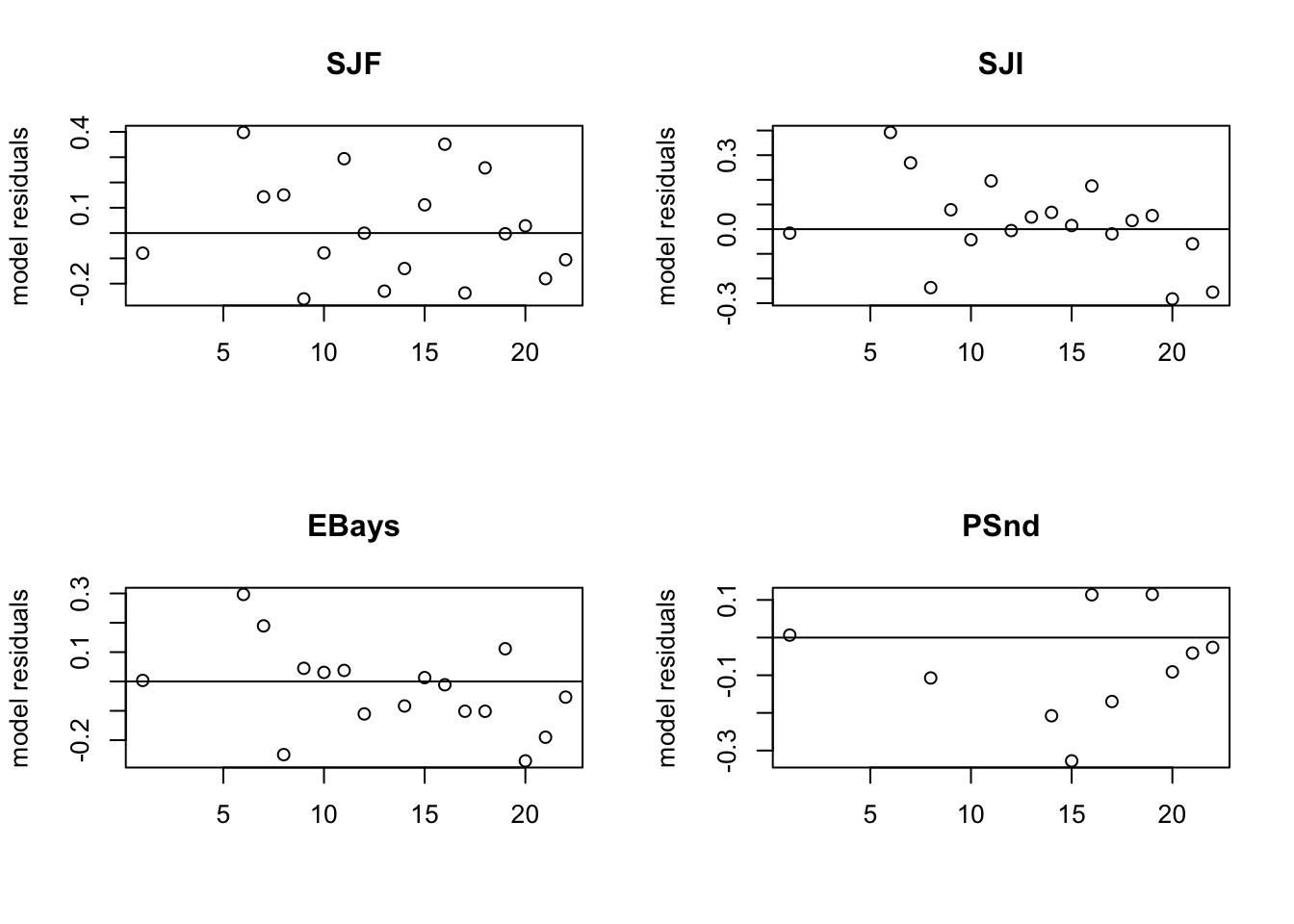

Figure 7.3: The model residuals for the model with four temporally correlated subpopulations.

Figure 7.4 shows the estimated states for each region using this code:

par(mfrow = c(2, 2))
for (i in 1:4) {
    plot(years, fit.2$states[i, ], ylab = "log subpopulation estimate", 
        xlab = "", type = "l")
    lines(years, fit.2$states[i, ] - 1.96 * fit.2$states.se[i, 
        ], type = "l", lwd = 1, lty = 2, col = "red")
    lines(years, fit.2$states[i, ] + 1.96 * fit.2$states.se[i, 
        ], type = "l", lwd = 1, lty = 2, col = "red")
    title(rownames(dat)[i])
}

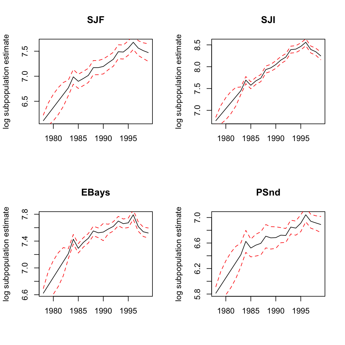
Figure 7.4: Plot of the estimate of log harbor seals in each region. The 95% confidence intervals on the population estimates are the dashed lines. These are not the confidence intervals on the observations, and the observations (the numbers) will not fall between the confidence interval lines.