7.9 Fitting a MARSS model with JAGS

Here we show you how to fit a MARSS model for the harbor seal data using JAGS. We will focus on four time series from inland Washington and set up the data as follows:

data(harborSealWA, package = "MARSS")
sites <- c("SJF", "SJI", "EBays", "PSnd")
Y <- harborSealWA[, sites]
Y <- t(Y)  # time across columns

We will fit the model with four temporally independent subpopulations with the same population growth rate (\(u\)) and year-to-year variance (\(q\)). This is the model in Section 7.4.

7.9.1 Writing the model in JAGS

The first step is to write this model in JAGS. See Chapter 12 for more information on and examples of JAGS models.

jagsscript <- cat("
model {  
   U ~ dnorm(0, 0.01);
   tauQ~dgamma(0.001,0.001);
   Q <- 1/tauQ;

   # Estimate the initial state vector of population abundances
   for(i in 1:nSites) {
      X[i,1] ~ dnorm(3,0.01); # vague normal prior 
   }

   # Autoregressive process for remaining years
   for(t in 2:nYears) {
      for(i in 1:nSites) {
         predX[i,t] <- X[i,t-1] + U;
         X[i,t] ~ dnorm(predX[i,t], tauQ);
      }
   }

   # Observation model
   # The Rs are different in each site
   for(i in 1:nSites) {
     tauR[i]~dgamma(0.001,0.001);
     R[i] <- 1/tauR[i];
   }
   for(t in 1:nYears) {
     for(i in 1:nSites) {
       Y[i,t] ~ dnorm(X[i,t],tauR[i]);
     }
   }
}  

", 
    file = "marss-jags.txt")

7.9.2 Fit the JAGS model

{#sec-mss-fit-jags}

Then we write the data list, parameter list, and pass the model to the jags() function:

jags.data <- list(Y = Y, nSites = nrow(Y), nYears = ncol(Y))  # named list
jags.params <- c("X", "U", "Q", "R")
model.loc <- "marss-jags.txt"  # name of the txt file
mod_1 <- jags(jags.data, parameters.to.save = jags.params, model.file = model.loc, 
    n.chains = 3, n.burnin = 5000, n.thin = 1, n.iter = 10000, 
    DIC = TRUE)

7.9.3 Plot the posteriors for the estimated states

We can plot any of the variables we chose to return to R in the jags.params list. Let’s focus on the X. When we look at the dimension of the X, we can use the apply() function to calculate the means and 95 percent CIs of the estimated states.

# attach.jags attaches the jags.params to our workspace
attach.jags(mod_1)
means <- apply(X, c(2, 3), mean)
upperCI <- apply(X, c(2, 3), quantile, 0.975)
lowerCI <- apply(X, c(2, 3), quantile, 0.025)
par(mfrow = c(2, 2))
nYears <- ncol(Y)
for (i in 1:nrow(means)) {
    plot(means[i, ], lwd = 3, ylim = range(c(lowerCI[i, ], upperCI[i, 
        ])), type = "n", main = colnames(Y)[i], ylab = "log abundance", 
        xlab = "time step")
    polygon(c(1:nYears, nYears:1, 1), c(upperCI[i, ], rev(lowerCI[i, 
        ]), upperCI[i, 1]), col = "skyblue", lty = 0)
    lines(means[i, ], lwd = 3)
    title(rownames(Y)[i])
}

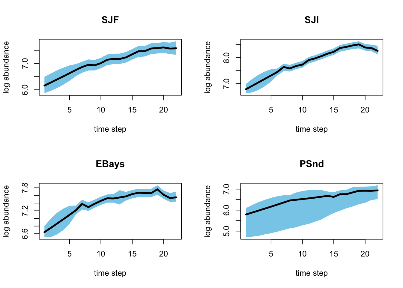
Figure 7.6: Plot of the posterior means and credible intervals for the estimated states.

detach.jags()