15.1 Overview

As discussed in Section 8.6.3 in the covariates chapter, we can model season with sine and cosine covariates.

\[y_t = x_t + \beta_1 \sin(2 \pi t/p) + \beta_2 \cos(2 \pi t/p) + e_t\] where \(t\) is the time step (1 to length of the time series) and \(p\) is the frequency of the data (e.g. 12 for monthly data). \(\alpha_t\) is the mean level about which the data \(y_t\) are fluctuating.

We can simulate data like this as follows:

set.seed(1234)
TT <- 100
q <- 0.1
r <- 0.1
beta1 <- 0.6
beta2 <- 0.4
cov1 <- sin(2 * pi * (1:TT)/12)
cov2 <- cos(2 * pi * (1:TT)/12)
xt <- cumsum(rnorm(TT, 0, q))
yt <- xt + beta1 * cov1 + beta2 * cov2 + rnorm(TT, 0, r)
plot(yt, type = "l", xlab = "t")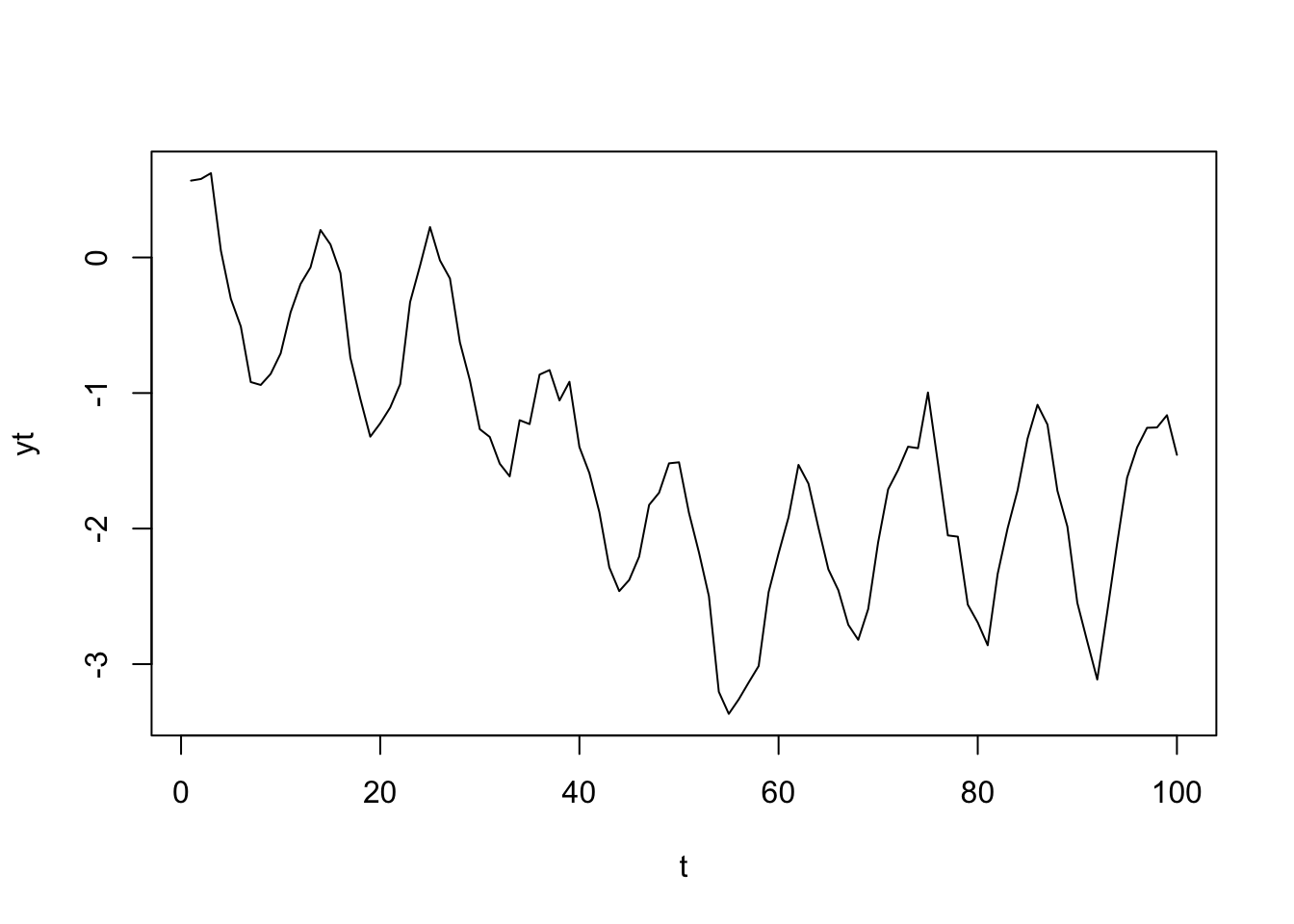

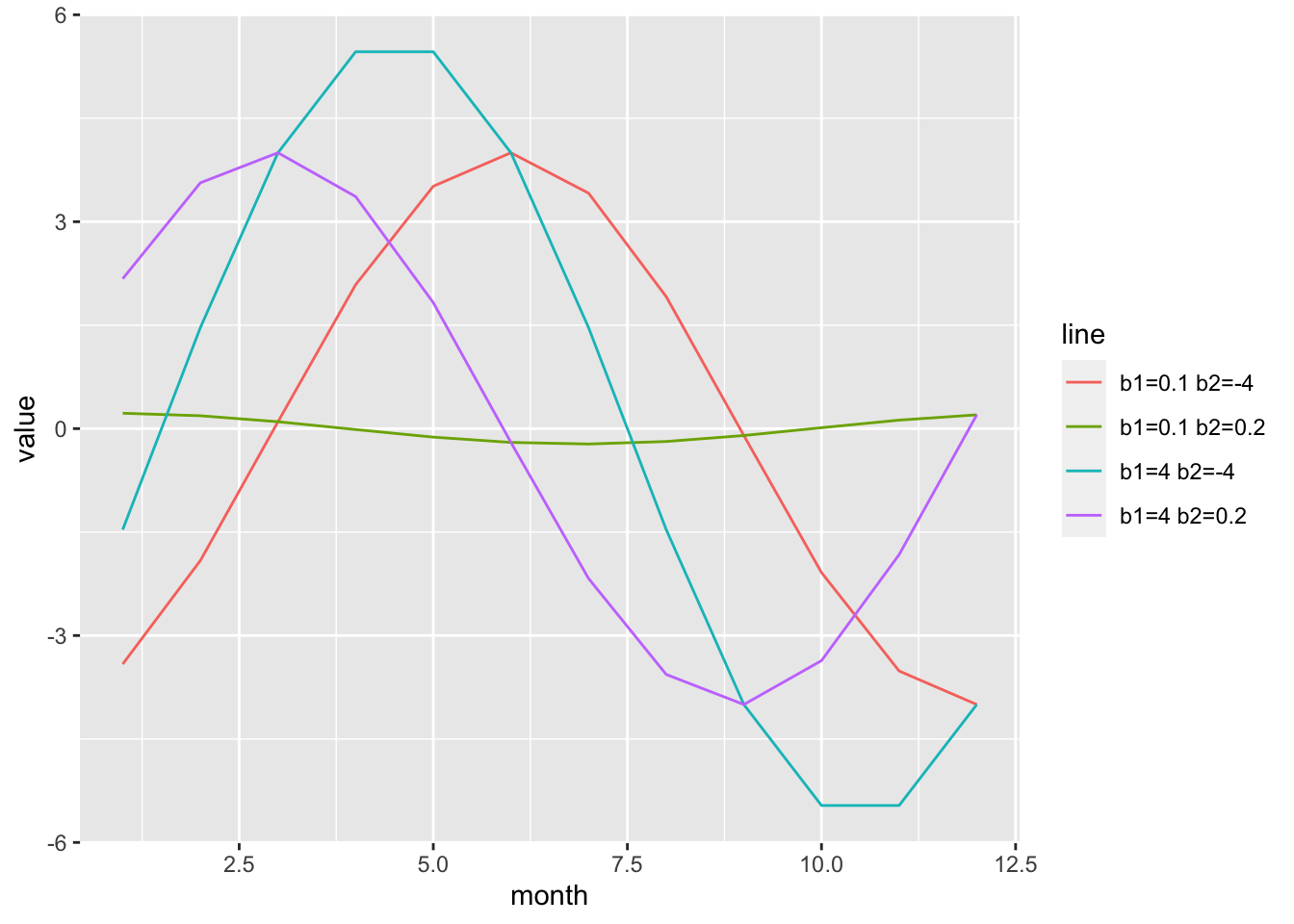
In this case, the seasonal cycle is constant over time since \(\beta_1\) and \(\beta_2\) are fixed (not varying in time).

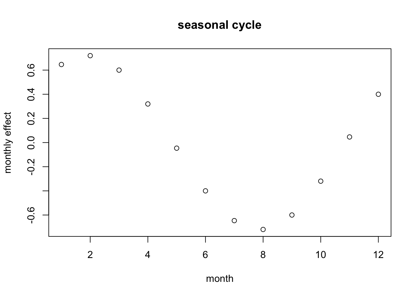
The \(\beta\) determine the shape and amplitude of the seasonal cycle—though in this case we will only have one peak per year.