16.5 Multivariate DLM 1: Synchrony in levels

In the first analysis, we will look at whether the stochastic levels (underlying trends) are correlated. We will analyze all the rivers together but in the equations, we will show just two rivers to keep the equations concise.

16.5.1 State model

The hidden states model will have the following components:

Each trend \(x\) will be modeled as separate but allowed to be correlated. This means either an unconstrained \(\mathbf{Q}\) or an equal variance and equal covariance matrix.
Each seasonal trend, the \(\beta\)’s, will also be treated as separate but independent. This means either a diagonal and equal variance \(\mathbf{Q}\) or diagona and unequal variances.

The \(\mathbf{x}\) equation is then:

\[\begin{bmatrix}x_a \\ x_b \\ \beta_{1a} \\ \beta_{1b} \\ \beta_{2a} \\ \beta_{2b} \end{bmatrix}_t = \begin{bmatrix}x_a \\ x_b \\ \beta_{1a} \\ \beta_{1b} \\ \beta_{2a} \\ \beta_{2b}\end{bmatrix}_{t-1} + \begin{bmatrix}w_1 \\ w_2 \\ w_3 \\ w_4 \\ w_5 \\ w_6 \end{bmatrix}_t\]

\[\begin{bmatrix}w_1 \\ w_2 \\ w_3 \\ w_4 \\ w_5 \\ w_6 \end{bmatrix}_t \sim \text{MVN}\left(0, \begin{bmatrix} q_a & c & 0 & 0 & 0 & 0\\ c & q_b & 0 & 0 & 0 & 0 \\ 0 & 0 & q_1 & 0 & 0 & 0 \\ 0 & 0 & 0 & q_2 & 0 & 0 \\ 0 & 0 & 0 & 0 & q_3 & 0 \\ 0 & 0 & 0 & 0 & 0 & q_4 \end{bmatrix}\right)\]

16.5.2 Observation model

The observation model will have the following components:

Each spawner count time series will be treated as independent with independent error (equal or unequal variance).

\[\begin{bmatrix}y_a \\ y_b\end{bmatrix}_t = \begin{bmatrix} 1 & 0 & \sin(2\pi t/p) & 0 & \cos(2\pi t/p) & 0\\ 0 & 1 & 0&\sin(2\pi t/p) & 0&\cos(2\pi t/p) \end{bmatrix} \begin{bmatrix} x_a \\ x_b \\ \beta_{1a} \\ \beta_{1b} \\ \beta_{2a} \\ \beta_{2b} \end{bmatrix}_t + \mathbf{v}_t\]

16.5.3 Fit model

Set the number of rivers.

n <- 2

The following code will create the \(\mathbf{Z}\) for a model with \(n\) rivers. The first \(\mathbf{Z}\) is shown.

Z <- array(1, dim = c(n, n * 3, TT))
Z[1:n, 1:n, ] <- diag(1, n)
for (t in 1:TT) {
    Z[, (n + 1):(2 * n), t] <- diag(sin(2 * pi * t/p), n)
    Z[, (2 * n + 1):(3 * n), t] <- diag(cos(2 * pi * t/p), n)
}
Z[, , 1]

     [,1] [,2]      [,3]      [,4]     [,5]     [,6]
[1,]    1    0 0.9510565 0.0000000 0.309017 0.000000
[2,]    0    1 0.0000000 0.9510565 0.000000 0.309017

And this code will make the \(\mathbf{Q}\) matrix:

Q <- matrix(list(0), 3 * n, 3 * n)
Q[1:n, 1:n] <- "c"
diag(Q) <- c(paste0("q", letters[1:n]), paste0("q", 1:(2 * n)))
Q

     [,1] [,2] [,3] [,4] [,5] [,6]
[1,] "qa" "c"  0    0    0    0   
[2,] "c"  "qb" 0    0    0    0   
[3,] 0    0    "q1" 0    0    0   
[4,] 0    0    0    "q2" 0    0   
[5,] 0    0    0    0    "q3" 0   
[6,] 0    0    0    0    0    "q4"

We will write a function to prepare the model matrices and fit. It takes the names of the rivers.

fitriver.m <- function(river, p = 5) {
    require(tidyr)
    require(dplyr)
    require(MARSS)
    df <- subset(sockeye, region %in% river)
    df <- df %>%
        pivot_wider(id_cols = brood_year, names_from = "region", 
            values_from = spawners) %>%
        ungroup() %>%
        select(-brood_year)
    yt <- t(log(df))
    TT <- ncol(yt)
    n <- nrow(yt)
    Z <- array(1, dim = c(n, n * 3, TT))
    Z[1:n, 1:n, ] <- diag(1, n)
    for (t in 1:TT) {
        Z[, (n + 1):(2 * n), t] <- diag(sin(2 * pi * t/p), n)
        Z[, (2 * n + 1):(3 * n), t] <- diag(cos(2 * pi * t/p), 
            n)
    }
    Q <- matrix(list(0), 3 * n, 3 * n)
    Q[1:n, 1:n] <- paste0("c", 1:(n^2))
    diag(Q) <- c(paste0("q", letters[1:n]), paste0("q", 1:(2 * 
        n)))
    Q[lower.tri(Q)] <- t(Q)[lower.tri(Q)]
    mod.list <- list(U = "zero", Q = Q, Z = Z, A = "zero")
    fit <- MARSS(yt, model = mod.list, inits = list(x0 = matrix(0, 
        3 * n, 1)), silent = TRUE)
    return(fit)
}

Now we can fit for two (or more) rivers. Note it didn’t quite converge as some of the variances for the \(\beta\)’s are going to 0 (constant \(\beta\) value).

river <- unique(sockeye$region)
n <- length(river)
fit <- fitriver.m(river)

16.5.4 Look at the results

We will look at the correlation plot for the trends.

require(corrplot)
Qmat <- coef(fit, type = "matrix")$Q[1:n, 1:n]
rownames(Qmat) <- colnames(Qmat) <- river
M <- cov2cor(Qmat)
corrplot(M, order = "hclust", addrect = 4)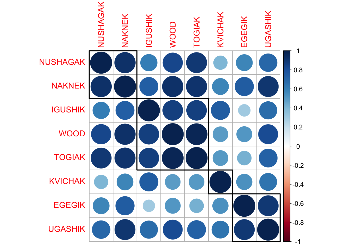

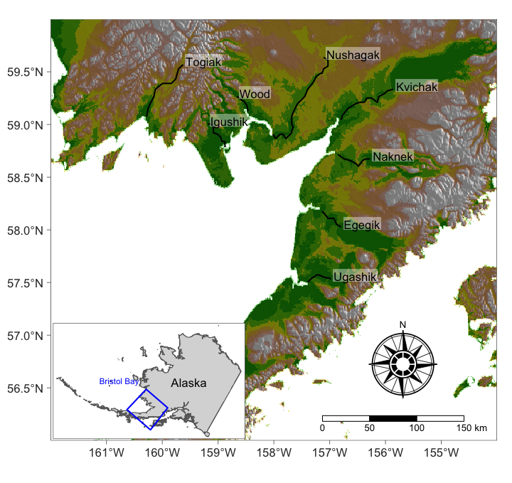
We can compare to the locations and see that this suggests that there is small scale regional correlation in the spawner counts.