6.3 The StructTS function

The StructTS function in the stats package in R will also fit the stochastic level model:

fit.sts <- StructTS(dat, type = "level")
fit.sts


Call:
StructTS(x = dat, type = "level")

Variances:
  level  epsilon  
   1469    15099

The estimates from StructTS() will be different (though similar) from MARSS() because StructTS() uses $x_1 = y_1$, that is the hidden state at $t=1$ is fixed to be the data at $t=1$. That is fine if you have a long data set, but would be disastrous for the short data sets typical in fisheries and ecology.

StructTS() is much, much faster for long time series. The example in ?StructTS is pretty much instantaneous with StructTS() but takes minutes with the EM algorithm that is the default in MARSS(). With the BFGS algorithm, it is much closer to StructTS():

trees <- window(treering, start = 0)
fitts <- StructTS(trees, type = "level")
fitem <- MARSS(trees, mod.nile.2)
fitbf <- MARSS(trees, mod.nile.2, method = "BFGS")

Note that mod.nile.2 specifies a univariate stochastic level model so we can use it just fine with other univariate data sets.

In addition, fitted(fit.sts) where fit.sts is a fit from StructTS() is very different than fit.marss$states from MARSS().

t <- 10
fitted(fit.sts)[t]

[1] 1162.904

is the expected value of $y_{t+1}$ (in this case $y_{11}$ since we set $t=10$) given the data up to $y_t$ (in this case, up to $y_{10}$). It is called the one-step ahead prediction.
We are not going to use the one-step ahead predictions unless we are forecasting or doing cross-validation.

Typically, when we analyze fisheries and ecological data, we want to know the estimate of the state, the $x_t$, given ALL the data (sometimes we might want the estimate of the $y_t$ process given all the data). For example, we might need an estimate of the population size in year 1990 given a time series of counts from 1930 to 2015. We don’t want to use only the data up to 1989; we want to use all the information. fit.marss$states from MARSS() is the expected value of $x_t$ given all the data. In the MARSS package, this is denoted “xtT.”

fitted(kem.2, type = "xtT") %>%
    subset(t == 11)

If you needed the one-step predictions from MARSS(), you can get that using “xtt1.”

fitted(kem.2, type = "xtt1") %>%
    subset(t == 11)

This is the expected value of $x_t$ conditioned on $y_1$ to $y_{t-1}$.

Loading required package: lattice

Loading required package: survival

Loading required package: Formula


Attaching package: 'Hmisc'

The following object is masked from 'package:quantmod':

    Lag

The following objects are masked from 'package:base':

    format.pval, units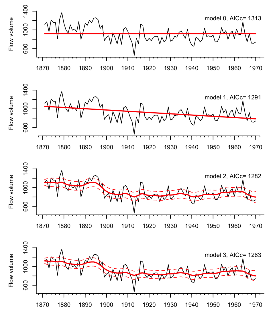

The Nile River flow volume with the model estimated flow rates (solid lines). The bottom model is a stochastic level model, meaning there isn’t one level line. Rather the level line is a distribution that has a mean and standard deviation. The solid state line in the bottom plots is the mean of the stochastic level and the 2 standard deviations are shown. The other two models are deterministic level models so the state is not stochastic and does not have a standard deviation.

Figure 6.2: The Nile River flow volume with the model estimated flow rates (solid lines). The bottom model is a stochastic level model, meaning there isn’t one level line. Rather the level line is a distribution that has a mean and standard deviation. The solid state line in the bottom plots is the mean of the stochastic level and the 2 standard deviations are shown. The other two models are deterministic level models so the state is not stochastic and does not have a standard deviation.