10.12 Example from Lake Washington
The Lake Washington dataset has two environmental covariates that we might expect to have effects on phytoplankton growth, and hence, abundance: temperature (Temp) and total phosphorous (TP). We need the covariate inputs to have the same number of time steps as the variate data, and thus we limit the covariate data to the years 1980-1994 also.
temp <- t(plank_dat[, "Temp", drop = FALSE])
TP <- t(plank_dat[, "TP", drop = FALSE])
We will now fit three different models that each add covariate effects (i.e., Temp, TP, Temp and TP) to our existing model above where \(m\) = 3 and \(\mathbf{R}\) is "diagonal and unequal".
mod_list = list(m = 3, R = "diagonal and unequal")
dfa_temp <- MARSS(dat, model = mod_list, form = "dfa", z.score = FALSE,
    control = con_list, covariates = temp)
dfa_TP <- MARSS(dat, model = mod_list, form = "dfa", z.score = FALSE,
    control = con_list, covariates = TP)
dfa_both <- MARSS(dat, model = mod_list, form = "dfa", z.score = FALSE,
    control = con_list, covariates = rbind(temp, TP))
Next we can compare whether the addition of the covariates improves the model fit.
print(cbind(model = c("no covars", "Temp", "TP", "Temp & TP"),
    AICc = round(c(dfa_1$AICc, dfa_temp$AICc, dfa_TP$AICc, dfa_both$AICc))),
    quote = FALSE)
model AICc
[1,] no covars 1427
[2,] Temp 1356
[3,] TP 1414
[4,] Temp & TP 1362This suggests that adding temperature or phosphorus to the model, either alone or in combination with one another, does seem to improve overall model fit. If we were truly interested in assessing the “best” model structure that includes covariates, however, we should examine all combinations of 1-4 trends and different structures for \(\mathbf{R}\).
Now let’s try to fit a model with a dummy variable for season, and see how that does.
cos_t <- cos(2 * pi * seq(TT)/12)
sin_t <- sin(2 * pi * seq(TT)/12)
dd <- rbind(cos_t, sin_t)
dfa_seas <- MARSS(dat, model = mod_list, form = "dfa", z.score = FALSE,
    control = con_list, covariates = dd)
Success! abstol and log-log tests passed at 451 iterations.
Alert: conv.test.slope.tol is 0.5.
Test with smaller values (<0.1) to ensure convergence.
MARSS fit is
Estimation method: kem
Convergence test: conv.test.slope.tol = 0.5, abstol = 0.001
Estimation converged in 451 iterations.
Log-likelihood: -633.1283
AIC: 1320.257 AICc: 1322.919
Estimate
Z.11 0.26207
Z.21 0.24762
Z.31 0.03689
Z.41 0.51329
Z.51 0.18479
Z.22 0.04819
Z.32 -0.08824
Z.42 0.06454
Z.52 0.05905
Z.33 0.02673
Z.43 0.19343
Z.53 -0.10528
R.(Cryptomonas,Cryptomonas) 0.14406
R.(Diatoms,Diatoms) 0.44205
R.(Greens,Greens) 0.73113
R.(Unicells,Unicells) 0.19533
R.(Other.algae,Other.algae) 0.50127
D.(Cryptomonas,cos_t) -0.23244
D.(Diatoms,cos_t) -0.40829
D.(Greens,cos_t) -0.72656
D.(Unicells,cos_t) -0.34666
D.(Other.algae,cos_t) -0.41606
D.(Cryptomonas,sin_t) 0.12515
D.(Diatoms,sin_t) 0.65621
D.(Greens,sin_t) -0.50657
D.(Unicells,sin_t) -0.00867
D.(Other.algae,sin_t) -0.62474
Initial states (x0) defined at t=0
Standard errors have not been calculated.
Use MARSSparamCIs to compute CIs and bias estimates.dfa_seas$AICc[1] 1322.919The model with a dummy seasonal factor does much better than the covariate models. The model fits for the seasonal effects model are shown below.
## get model fits & CI's
mod_fit <- get_DFA_fits(dfa_seas, dd = dd)
## plot the fits
ylbl <- phytoplankton
par(mfrow = c(N_ts, 1), mai = c(0.5, 0.7, 0.1, 0.1), omi = c(0,
    0, 0, 0))
for (i in 1:N_ts) {
    up <- mod_fit$up[i, ]
    mn <- mod_fit$ex[i, ]
    lo <- mod_fit$lo[i, ]
    plot(w_ts, mn, xlab = "", ylab = ylbl[i], xaxt = "n", type = "n",
        cex.lab = 1.2, ylim = c(min(lo), max(up)))
    axis(1, 12 * (0:dim(dat_1980)[2]) + 1, yr_frst + 0:dim(dat_1980)[2])
    points(w_ts, dat[i, ], pch = 16, col = clr[i])
    lines(w_ts, up, col = "darkgray")
    lines(w_ts, mn, col = "black", lwd = 2)
    lines(w_ts, lo, col = "darkgray")
}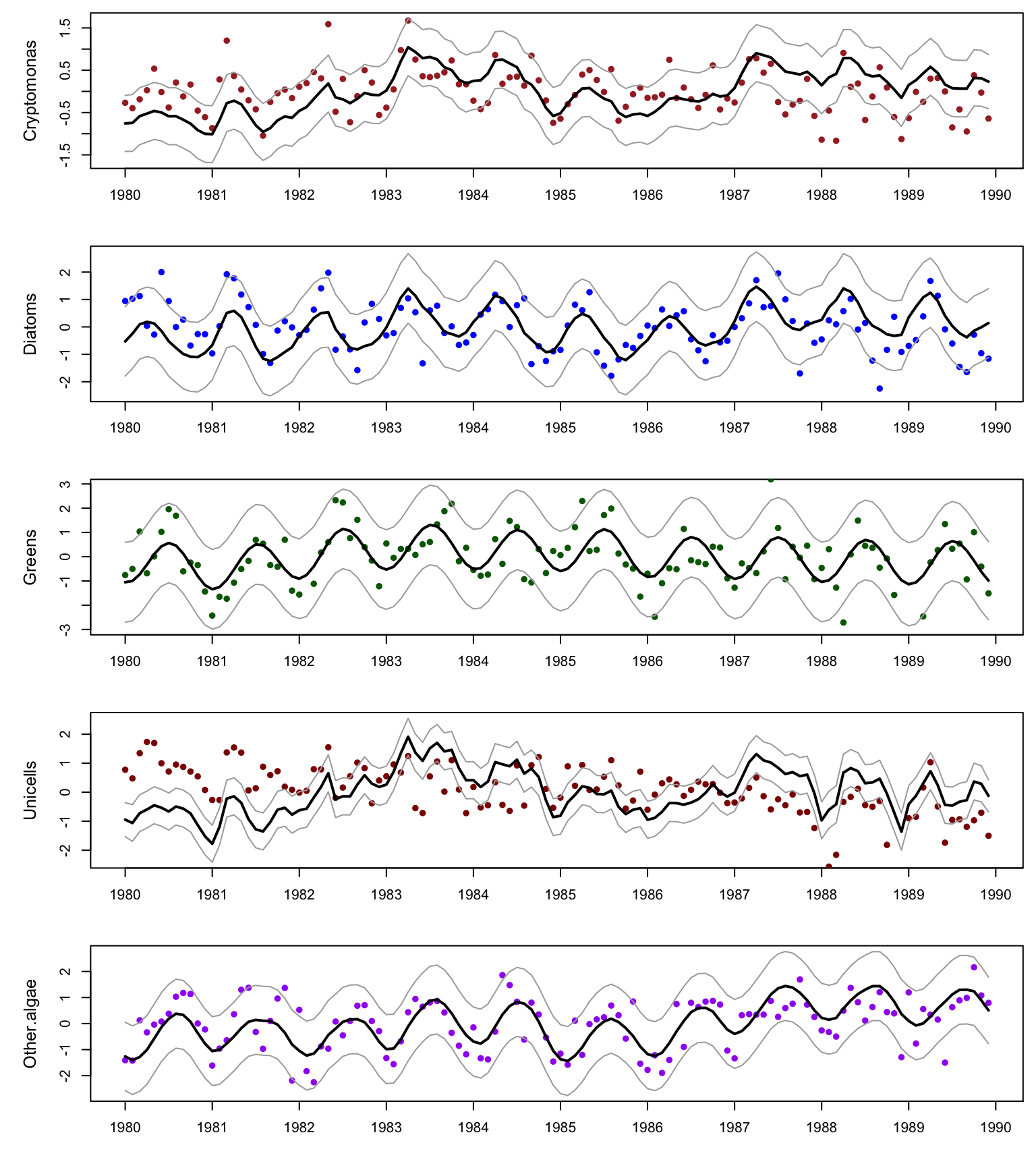
Figure 10.5: Data and model fits for the DFA with covariates.