4.3 Differencing to remove a trend or seasonal effects
An alternative to decomposition for removing trends is differencing. We saw in lecture how the difference operator works and how it can be used to remove linear and nonlinear trends as well as various seasonal features that might be evident in the data. As a reminder, we define the difference operator as
\[\begin{equation} \tag{4.6} \nabla x_t = x_t - x_{t-1}, \end{equation}\]
and, more generally, for order \(d\)
\[\begin{equation} \tag{4.7} \nabla^d x_t = (1-\mathbf{B})^d x_t, \end{equation}\] where B is the backshift operator (i.e., \(\mathbf{B}^k x_t = x_{t-k}\) for \(k \geq 1\)).
So, for example, a random walk is one of the most simple and widely used time series models, but it is not stationary. We can write a random walk model as
\[\begin{equation} \tag{4.8} x_t = x_{t-1} + w_t, \text{ with } w_t \sim \text{N}(0,q). \end{equation}\]
Applying the difference operator to Equation (4.8) will yield a time series of Gaussian white noise errors \(\{w_t\}\):
\[\begin{equation} \tag{4.9} \begin{aligned} \nabla (x_t &= x_{t-1} + w_t) \\ x_t - x_{t-1} &= x_{t-1} - x_{t-1} + w_t \\ x_t - x_{t-1} &= w_t \end{aligned} \end{equation}\]
4.3.1 Using the diff() function
In R we can use the diff() function for differencing a time series, which requires 3 arguments: x (the data), lag (the lag at which to difference), and differences (the order of differencing; \(d\) in Equation (4.7)). For example, first-differencing a time series will remove a linear trend (i.e., differences = 1); twice-differencing will remove a quadratic trend (i.e., differences = 2). In addition, first-differencing a time series at a lag equal to the period will remove a seasonal trend (e.g., set lag = 12 for monthly data).
Let’s use diff() to remove the trend and seasonal signal from the CO\(_2\) time series, beginning with the trend. Close inspection of Figure 4.1 would suggest that there is a nonlinear increase in CO\(_2\) concentration over time, so we’ll set differences = 2):
## twice-difference the CO2 data
co2_d2 <- diff(co2, differences = 2)
## plot the differenced data
plot(co2_d2, ylab = expression(paste(nabla^2, "CO"[2])))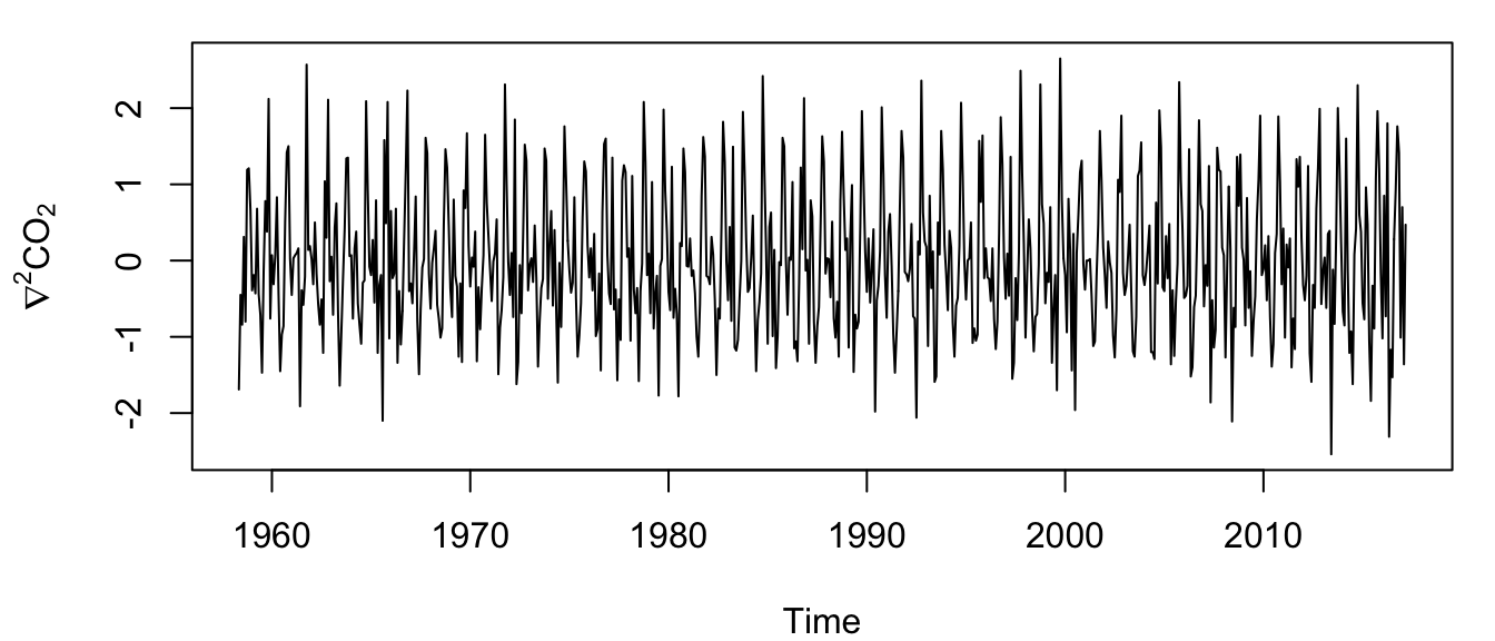
Figure 4.8: Time series of the twice-differenced atmospheric CO\(_2\) concentration at Mauna Loa, Hawai’i.
We were apparently successful in removing the trend, but the seasonal effect still appears obvious (Figure 4.8). Therefore, let’s go ahead and difference that series at lag-12 because our data were collected monthly.
## difference the differenced CO2 data
co2_d2d12 <- diff(co2_d2, lag = 12)
## plot the newly differenced data
plot(co2_d2d12, ylab = expression(paste(nabla, "(", nabla^2,
    "CO"[2], ")")))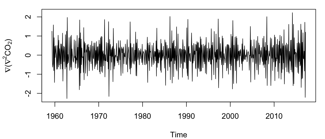
Figure 4.9: Time series of the lag-12 difference of the twice-differenced atmospheric CO\(_2\) concentration at Mauna Loa, Hawai’i.
Now we have a time series that appears to be random errors without any obvious trend or seasonal components (Figure 4.9).