10.10 Plotting the data and model fits

We can plot the fits for our DFA model along with the data. The following function will return the fitted values ± (1-\(\alpha\))% confidence intervals.

get_DFA_fits <- function(MLEobj, dd = NULL, alpha = 0.05) {
    ## empty list for results
    fits <- list()
    ## extra stuff for var() calcs
    Ey <- MARSS:::MARSShatyt(MLEobj)
    ## model params
    ZZ <- coef(MLEobj, type = "matrix")$Z
    ## number of obs ts
    nn <- dim(Ey$ytT)[1]
    ## number of time steps
    TT <- dim(Ey$ytT)[2]
    ## get the inverse of the rotation matrix
    H_inv <- varimax(ZZ)$rotmat
    ## check for covars
    if (!is.null(dd)) {
        DD <- coef(MLEobj, type = "matrix")$D
        ## model expectation
        fits$ex <- ZZ %*% H_inv %*% MLEobj$states + DD %*% dd
    } else {
        ## model expectation
        fits$ex <- ZZ %*% H_inv %*% MLEobj$states
    }
    ## Var in model fits
    VtT <- MARSSkfss(MLEobj)$VtT
    VV <- NULL
    for (tt in 1:TT) {
        RZVZ <- coef(MLEobj, type = "matrix")$R - ZZ %*% VtT[, 
            , tt] %*% t(ZZ)
        SS <- Ey$yxtT[, , tt] - Ey$ytT[, tt, drop = FALSE] %*% 
            t(MLEobj$states[, tt, drop = FALSE])
        VV <- cbind(VV, diag(RZVZ + SS %*% t(ZZ) + ZZ %*% t(SS)))
    }
    SE <- sqrt(VV)
    ## upper & lower (1-alpha)% CI
    fits$up <- qnorm(1 - alpha/2) * SE + fits$ex
    fits$lo <- qnorm(alpha/2) * SE + fits$ex
    return(fits)
}

Here are time series of the five phytoplankton groups (points) with the mean of the DFA fits (black line) and the 95% confidence intervals (gray lines).

## get model fits & CI's
mod_fit <- get_DFA_fits(dfa_1)
## plot the fits
ylbl <- phytoplankton
par(mfrow = c(N_ts, 1), mai = c(0.5, 0.7, 0.1, 0.1), omi = c(0, 
    0, 0, 0))
for (i in 1:N_ts) {
    up <- mod_fit$up[i, ]
    mn <- mod_fit$ex[i, ]
    lo <- mod_fit$lo[i, ]
    plot(w_ts, mn, xlab = "", ylab = ylbl[i], xaxt = "n", type = "n", 
        cex.lab = 1.2, ylim = c(min(lo), max(up)))
    axis(1, 12 * (0:dim(dat_1980)[2]) + 1, yr_frst + 0:dim(dat_1980)[2])
    points(w_ts, dat[i, ], pch = 16, col = clr[i])
    lines(w_ts, up, col = "darkgray")
    lines(w_ts, mn, col = "black", lwd = 2)
    lines(w_ts, lo, col = "darkgray")
}

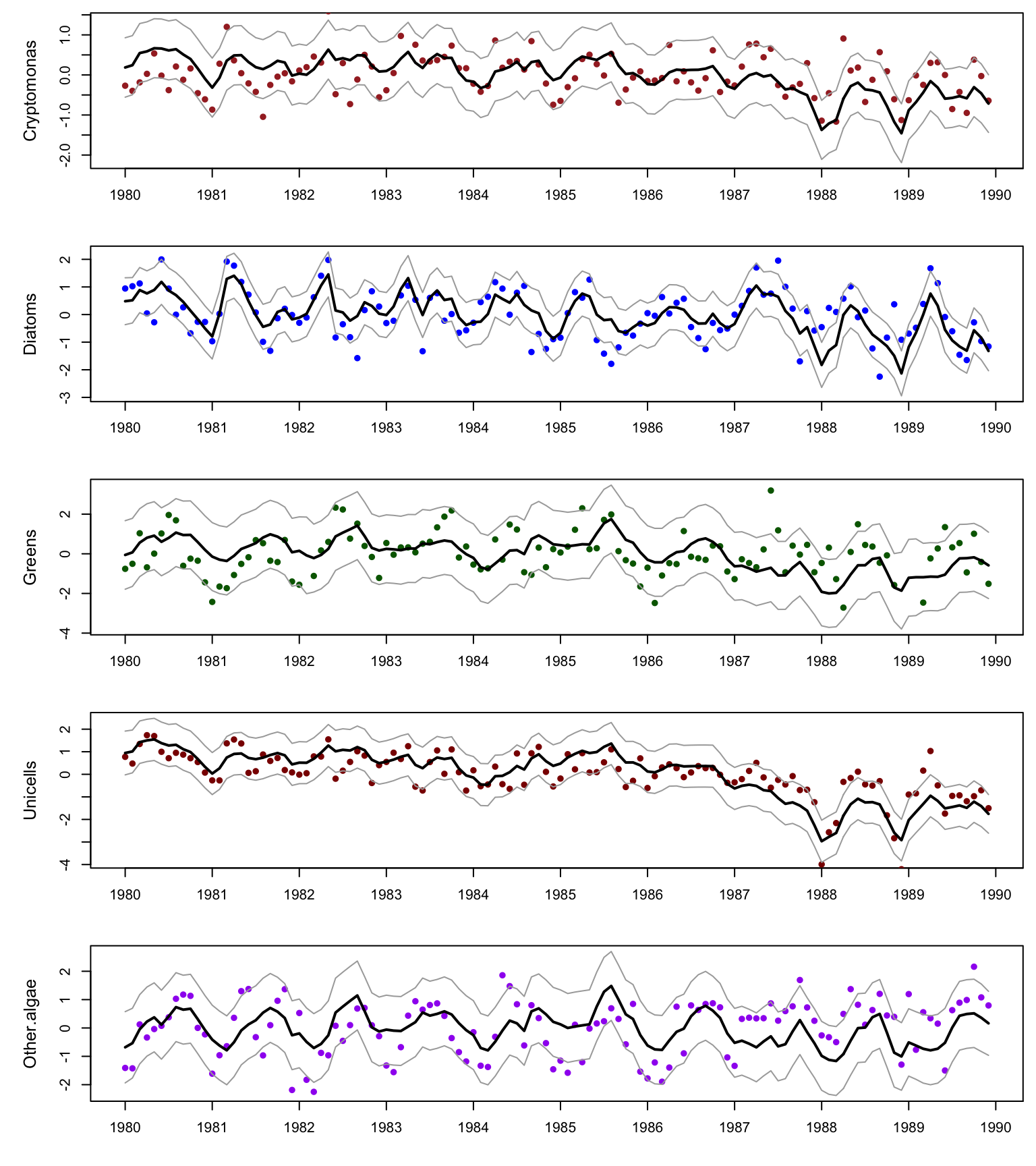
Figure 10.4: Data and fits from the DFA model.