3.7 Decomposition on log-transformed data
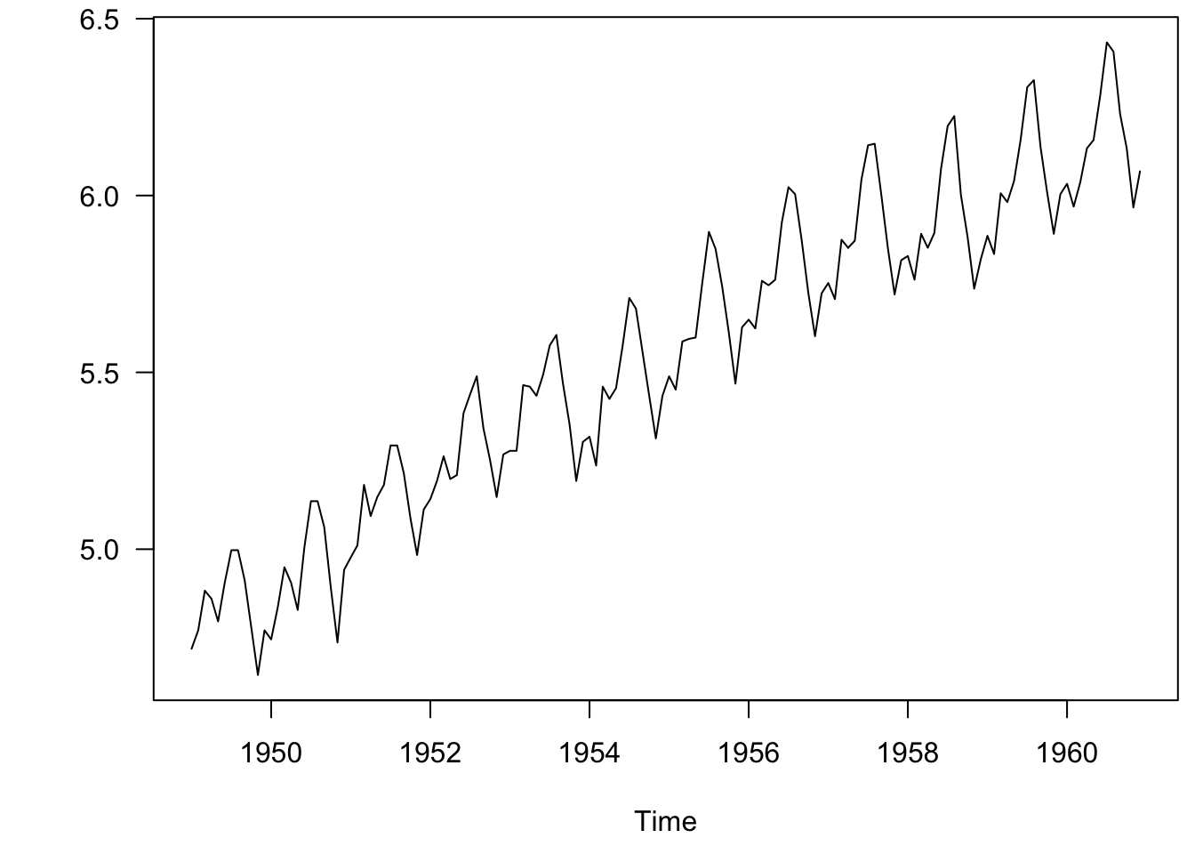
Let’s repeat the decomposition with the log of the airline data.
lx <- log(AirPassengers)
par(mai = c(0.9, 0.9, 0.1, 0.1), omi = c(0, 0, 0, 0))
plot.ts(lx, las = 1, ylab = "")
Figure 3.11: Log monthly airline passengers from 1949-1960
3.7.1 The trend (\(m_t\))

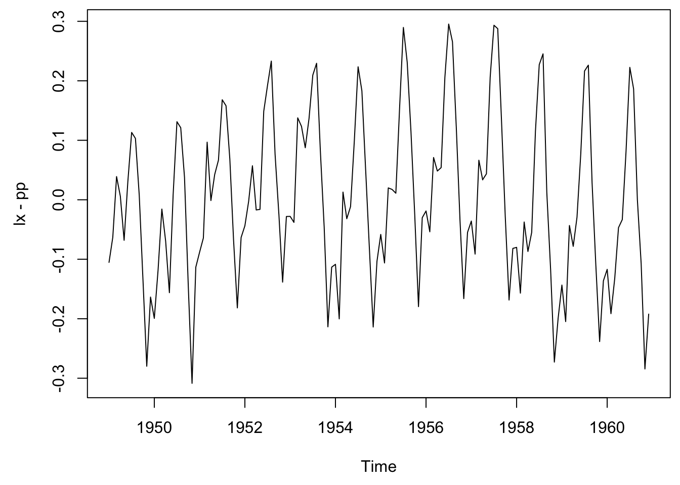
3.7.2 Seasonal effect (\(s_t\)) with error (\(e_t\))

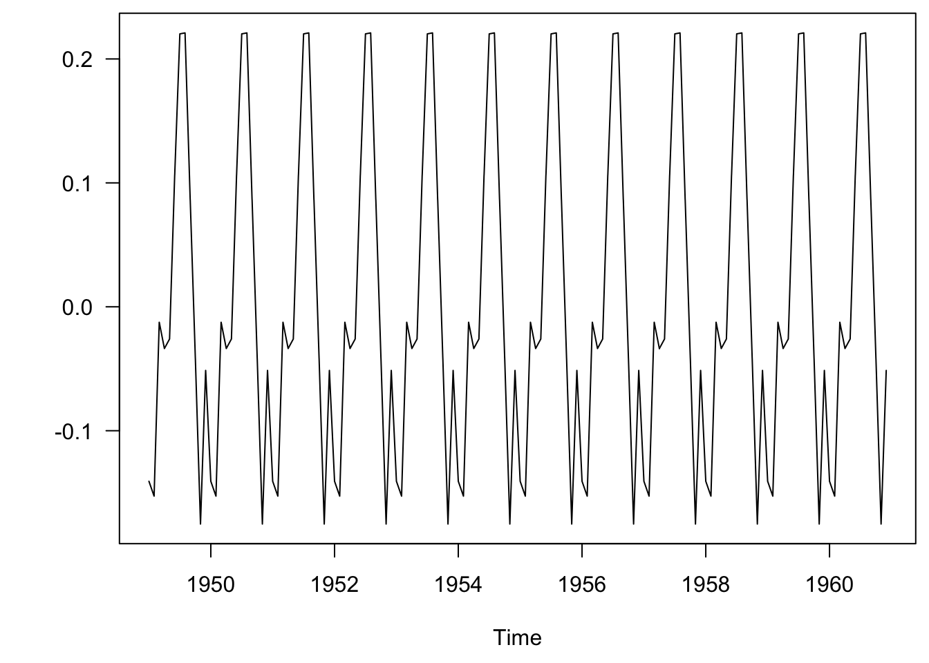
3.7.3 Mean seasonal effect (\(s_t\))

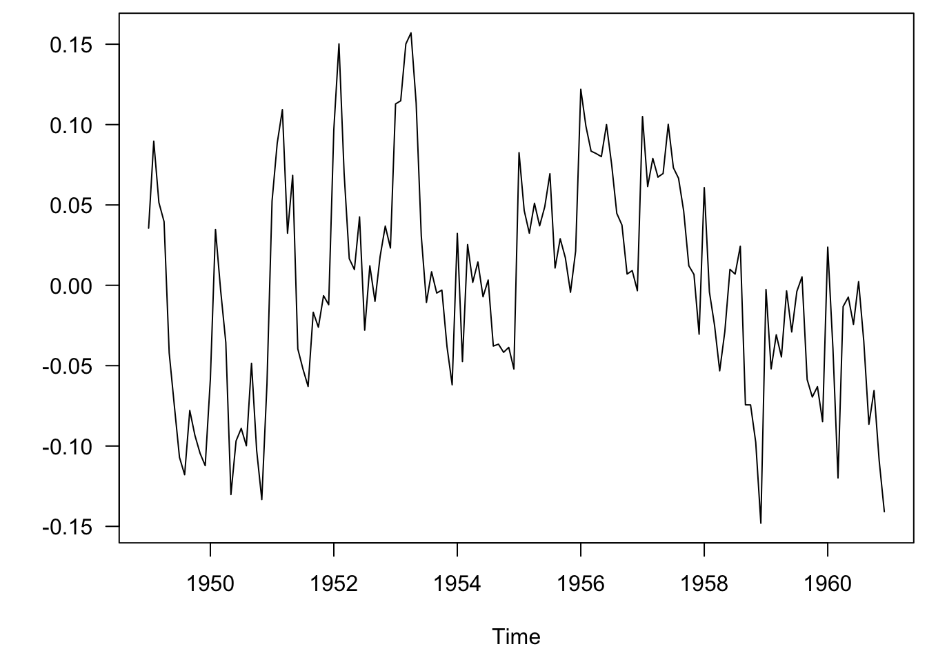
3.7.4 Remainder (\(e_t\))
le <- lx - pp - seas_2
par(mai = c(0.9, 0.9, 0.1, 0.1), omi = c(0, 0, 0, 0))
plot.ts(le, las = 1, ylab = "")