11.3 Modeling Seasonal SWE

When we look at all months, we see that SWE is highly seasonal. Note October and November are missing for all years.

swe.yr <- snotel
swe.yr <- swe.yr[swe.yr$Station.Id %in% y$Station.Id, ]
swe.yr$Station <- droplevels(swe.yr$Station)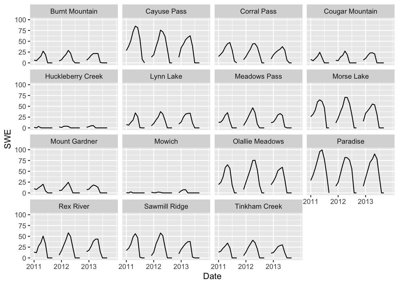

Set up the data matrix of monthly SNOTEL data:

dat.yr <- snotel
dat.yr <- dat.yr[dat.yr$Station.Id %in% y$Station.Id, ]
dat.yr$Station <- droplevels(dat.yr$Station)
dat.yr$Month <- factor(dat.yr$Month, level = month.abb)
dat.yr <- reshape2::acast(dat.yr, Station ~ Year + Month, value.var = "SWE")

We will model the seasonal differences using a periodic model. The covariates are

period <- 12
TT <- dim(dat.yr)[2]
cos.t <- cos(2 * pi * seq(TT)/period)
sin.t <- sin(2 * pi * seq(TT)/period)
c.seas <- rbind(cos.t, sin.t)

11.3.1 Modeling season across sites

We will create a state for the seasonal cycle and each station will have a scaled effect of that seasonal cycle. The observations will have the seasonal effect plus a mean and residuals (observation - season - mean) will be allowed to correlate across stations.

ns <- dim(dat.yr)[1]
B <- "zero"
Q <- matrix(1)
R <- "unconstrained"
U <- "zero"
x0 <- "zero"
Z <- matrix(paste0("z", 1:ns), ns, 1)
A <- "unequal"
mod.list.dfa = list(B = B, Z = Z, Q = Q, R = R, U = U, A = A, 
    x0 = x0)
C <- matrix(c("c1", "c2"), 1, 2)
c <- c.seas
mod.list.seas <- list(B = B, U = U, Q = Q, A = A, R = R, Z = Z, 
    C = C, c = c, x0 = x0, tinitx = 0)

Now we can fit the model:

m <- apply(dat.yr, 1, mean, na.rm = TRUE)
fit.seas <- MARSS(dat.yr, model = mod.list.seas, control = list(maxit = 500), 
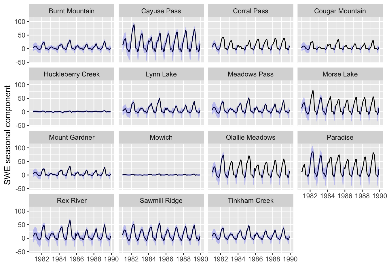
    inits = list(A = matrix(m, ns, 1)))

The seasonal patterns

Figure @ref{fig:mssmiss-seas} shows the seasonal estimate plus prediction intervals for each station. This is \(z_i x_i + a_i\). The prediction interval shows our estimate of the range of the data we would see around the seasonal estimate.

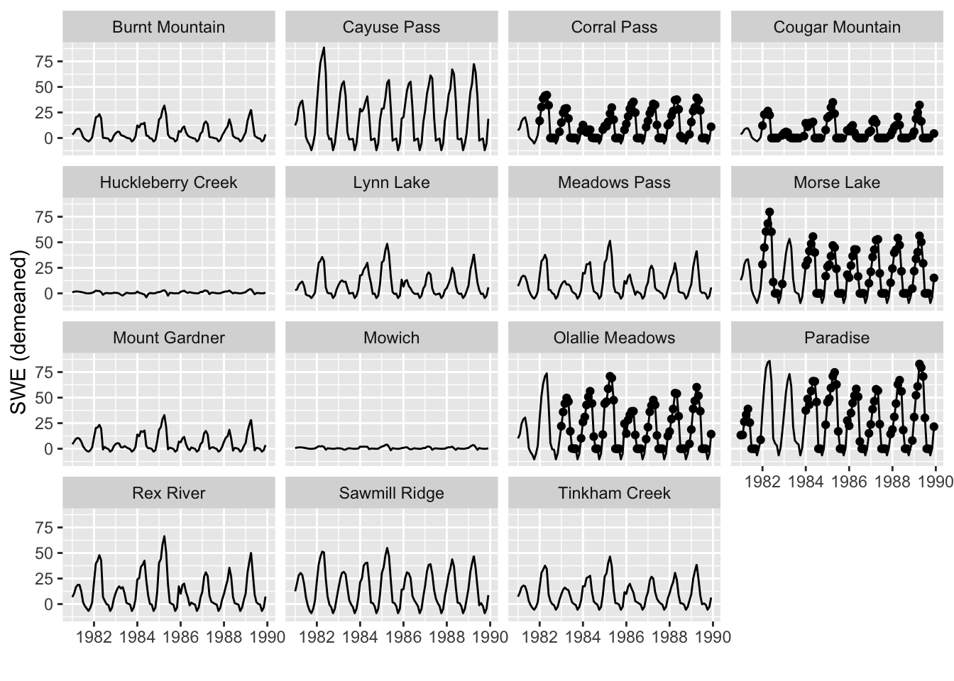
Estimates for the missing years

The estimated mean SWE at each station is \(E(y_{t,i}|y_{1:T})\). This is the estimate of \(y_{t,i}\) conditioned on all the data and includes the seasonal component plus the information from the data from other stations. If \(y_{t,i}\) is observed, \(E(y_{t,i}|y_{1:T}) = y_{t,i}\), i.e. just the observed value. But if \(y_{t,i}\) is unobserved, the stations with data at time \(t\) help inform \(y_{t,i}\), the value of the station without data at time \(t\). Note this is not the case when we computed the fitted value for \(y_{t,i}\). In that case, the data inform \(\mathbf{R}\) but we do not treat the observed data at \(t=i\) as ‘observed’ and influencing the missing the missing \(y_{t,i}\) through \(\mathbf{R}\).

Only years up to 1990 are shown, but the model is fit to all years. The stations with no data before 1990 are being estimated based on the information in the later years when they do have data. We did not constrain the SWE to be positive, so negative estimates are possible and occurs in the months in which we have no SWE data (because there is no snow).