4.5 White noise (WN)
A time series \(\{w_t\}\) is a discrete white noise series (DWN) if the \(w_1, w_1, \dots, w_t\) are independent and identically distributed (IID) with a mean of zero. For most of the examples in this course we will assume that the \(w_t \sim \text{N}(0,q)\), and therefore we refer to the time series \(\{w_t\}\) as Gaussian white noise. If our time series model has done an adequate job of removing all of the serial autocorrelation in the time series with trends, seasonal effects, etc., then the model residuals (\(e_t = y_t - \hat{y}_t\)) will be a WN sequence with the following properties for its mean (\(\bar{e}\)), covariance (\(c_k\)), and autocorrelation (\(r_k\)):
\[\begin{equation} \tag{4.17} \begin{aligned} \bar{x} &= 0 \\ c_k &= \text{Cov}(e_t,e_{t+k}) = \begin{cases} q & \text{if } k = 0 \\ 0 & \text{if } k \neq 1 \end{cases} \\ r_k &= \text{Cor}(e_t,e_{t+k}) = \begin{cases} 1 & \text{if } k = 0 \\ 0 & \text{if } k \neq 1. \end{cases} \end{aligned} \end{equation}\]
4.5.1 Simulating white noise
Simulating WN in R is straightforward with a variety of built-in random number generators for continuous and discrete distributions. Once you know R’s abbreviation for the distribution of interest, you add an \(\texttt{r}\) to the beginning to get the function’s name. For example, a Gaussian (or normal) distribution is abbreviated \(\texttt{norm}\) and so the function is rnorm(). All of the random number functions require two things: the number of samples from the distribution and the parameters for the distribution itself (e.g., mean & SD of a normal). Check the help file for the distribution of interest to find out what parameters you must specify (e.g., type ?rnorm to see the help for a normal distribution).
Here’s how to generate 100 samples from a normal distribution with mean of 5 and standard deviation of 0.2, and 50 samples from a Poisson distribution with a rate (\(\lambda\)) of 20.
set.seed(123)
## random normal variates
GWN <- rnorm(n = 100, mean = 5, sd = 0.2)
## random Poisson variates
PWN <- rpois(n = 50, lambda = 20)
Here are plots of the time series. Notice that on one occasion the same number was drawn twice in a row from the Poisson distribution, which is discrete. That is virtually guaranteed to never happen with a continuous distribution.
## set up plot region
par(mfrow = c(1, 2))
## plot normal variates with mean
plot.ts(GWN)
abline(h = 5, col = "blue", lty = "dashed")
## plot Poisson variates with mean
plot.ts(PWN)
abline(h = 20, col = "blue", lty = "dashed")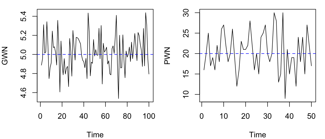
Figure 4.18: Time series plots of simulated Gaussian (left) and Poisson (right) white noise.
Now let’s examine the ACF for the 2 white noise series and see if there is, in fact, zero autocorrelation for lags \(\geq\) 1.
## set up plot region
par(mfrow = c(1, 2))
## plot normal variates with mean
acf(GWN, main = "", lag.max = 20)
## plot Poisson variates with mean
acf(PWN, main = "", lag.max = 20)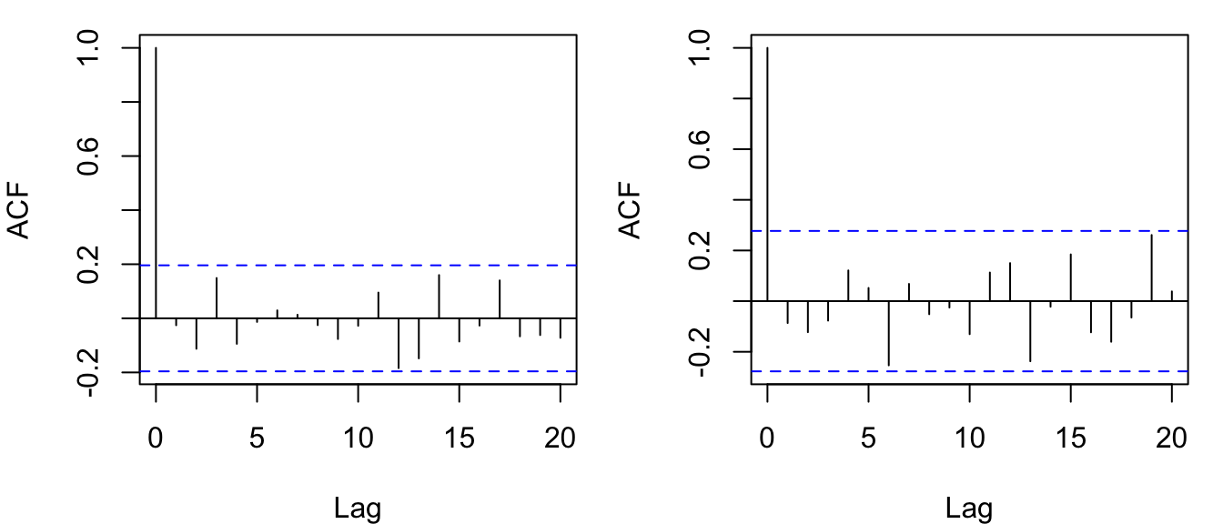
Figure 4.19: ACF’s for the simulated Gaussian (left) and Poisson (right) white noise shown in Figure 4.18.
Interestingly, the \(r_k\) are all greater than zero in absolute value although they are not statistically different from zero for lags 1-20. This is because we are dealing with a sample of the distributions rather than the entire population of all random variates. As an exercise, try setting n = 1e6 instead of n = 100 or n = 50 in the calls calls above to generate the WN sequences and see what effect it has on the estimation of \(r_k\). It is also important to remember, as we discussed earlier, that we should expect that approximately 1 in 20 of the \(r_k\) will be statistically greater than zero based on chance alone, especially for relatively small sample sizes, so don’t get too excited if you ever come across a case like then when inspecting model residuals.