8.6 Including seasonal effects in MARSS models

Time-series data are often collected at intervals with some implicit ``seasonality.’’ For example, quarterly earnings for a business, monthly rainfall totals, or hourly air temperatures. In those cases, it is often helpful to extract any recurring seasonal patterns that might otherwise mask some of the other temporal dynamics we are interested in examining.

Here we show a few approaches for including seasonal effects using the Lake Washington plankton data, which were collected monthly. The following examples will use all five phytoplankton species from Lake Washington. First, let’s set up the data.

years <- fulldat[, "Year"] >= 1965 & fulldat[, "Year"] < 1975
phytos <- c("Diatoms", "Greens", "Bluegreens", "Unicells", "Other.algae")
dat <- t(fulldat[years, phytos])

# z.score data because we changed the mean when we
# subsampled
the.mean <- apply(dat, 1, mean, na.rm = TRUE)
the.sigma <- sqrt(apply(dat, 1, var, na.rm = TRUE))
dat <- (dat - the.mean) * (1/the.sigma)
# number of time periods/samples
TT <- dim(dat)[2]

8.6.1 Seasonal effects as fixed factors

One common approach for estimating seasonal effects is to treat each one as a fixed factor, such that the number of parameters equals the number of ``seasons’’ (e.g., 24 hours per day, 4 quarters per year). The plankton data are collected monthly, so we will treat each month as a fixed factor. To fit a model with fixed month effects, we create a \(12 \times T\) covariate matrix \(\mathbf{c}\) with one row for each month (Jan, Feb, …) and one column for each time point. We put a 1 in the January row for each column corresponding to a January time point, a 1 in the February row for each column corresponding to a February time point, and so on. All other values of \(\mathbf{c}\) equal 0. The following code will create such a \(\mathbf{c}\) matrix.

# number of 'seasons' (e.g., 12 months per year)
period <- 12
# first 'season' (e.g., Jan = 1, July = 7)
per.1st <- 1
# create factors for seasons
c.in <- diag(period)
for (i in 2:(ceiling(TT/period))) {
    c.in <- cbind(c.in, diag(period))
}
# trim c.in to correct start & length
c.in <- c.in[, (1:TT) + (per.1st - 1)]
# better row names
rownames(c.in) <- month.abb

Next we need to set up the form of the \(\mathbf{C}\) matrix which defines any constraints we want to set on the month effects. \(\mathbf{C}\) is a \(5 \times 12\) matrix. Five taxon and 12 month effects. If we wanted each taxon to have the same month effect, i.e. there is a common month effect across all taxon, then we have the same value in each \(\mathbf{C}\) column:

C <- matrix(month.abb, 5, 12, byrow = TRUE)
C

     [,1]  [,2]  [,3]  [,4]  [,5]  [,6]  [,7]  [,8]  [,9]  [,10] [,11] [,12]
[1,] "Jan" "Feb" "Mar" "Apr" "May" "Jun" "Jul" "Aug" "Sep" "Oct" "Nov" "Dec"
[2,] "Jan" "Feb" "Mar" "Apr" "May" "Jun" "Jul" "Aug" "Sep" "Oct" "Nov" "Dec"
[3,] "Jan" "Feb" "Mar" "Apr" "May" "Jun" "Jul" "Aug" "Sep" "Oct" "Nov" "Dec"
[4,] "Jan" "Feb" "Mar" "Apr" "May" "Jun" "Jul" "Aug" "Sep" "Oct" "Nov" "Dec"
[5,] "Jan" "Feb" "Mar" "Apr" "May" "Jun" "Jul" "Aug" "Sep" "Oct" "Nov" "Dec"

Notice, that \(\mathbf{C}\) only has 12 values in it, the 12 common month effects. However, for this example, we will let each taxon have a different month effect thus allowing different seasonality for each taxon. For this model, we want each value in \(\mathbf{C}\) to be unique:

C <- "unconstrained"

Now \(\mathbf{C}\) has 5 \(\times\) 12 = 60 separate effects.

Then we set up the form for the rest of the model parameters. We make the following assumptions:

# Each taxon has unique density-dependence
B <- "diagonal and unequal"
# Assume independent process errors
Q <- "diagonal and unequal"
# We have demeaned the data & are fitting a mean-reverting
# model by estimating a diagonal B, thus
U <- "zero"
# Each obs time series is associated with only one process
Z <- "identity"
# The data are demeaned & fluctuate around a mean
A <- "zero"
# We assume observation errors are independent, but they
# have similar variance due to similar collection methods
R <- "diagonal and equal"
# We are not including covariate effects in the obs
# equation
D <- "zero"
d <- "zero"

Now we can set up the model list for MARSS and fit the model (results are not shown since they are verbose with 60 different month effects).

model.list <- list(B = B, U = U, Q = Q, Z = Z, A = A, R = R, 
    C = C, c = c.in, D = D, d = d)
seas.mod.1 <- MARSS(dat, model = model.list, control = list(maxit = 1500))

# Get the estimated seasonal effects rows are taxa, cols
# are seasonal effects
seas.1 <- coef(seas.mod.1, type = "matrix")$C
rownames(seas.1) <- phytos
colnames(seas.1) <- month.abb

The top panel in Figure 8.2 shows the estimated seasonal effects for this model. Note that if we had set U=“unequal,” we would need to set one of the columns of \(\mathbf{C}\) to zero because the model would be under-determined (infinite number of solutions). If we substracted the mean January abundance off each time series, we could set the January column in \(\mathbf{C}\) to 0 and get rid of 5 estimated effects.

8.6.2 Seasonal effects as a polynomial

The fixed factor approach required estimating 60 effects. Another approach is to model the month effect as a 3rd-order (or higher) polynomial: \(a+b\times m + c\times m^2 + d \times m^3\) where \(m\) is the month number. This approach has less flexibility but requires only 20 estimated parameters (i.e., 4 regression parameters times 5 taxa). To do so, we create a \(4 \times T\) covariate matrix \(\mathbf{c}\) with the rows corresponding to 1, \(m\), \(m^2\), and \(m^3\), and the columns again corresponding to the time points. Here is how to set up this matrix:

# number of 'seasons' (e.g., 12 months per year)
period <- 12
# first 'season' (e.g., Jan = 1, July = 7)
per.1st <- 1
# order of polynomial
poly.order <- 3
# create polynomials of months
month.cov <- matrix(1, 1, period)
for (i in 1:poly.order) {
    month.cov = rbind(month.cov, (1:12)^i)
}
# our c matrix is month.cov replicated once for each year
c.m.poly <- matrix(month.cov, poly.order + 1, TT + period, byrow = FALSE)
# trim c.in to correct start & length
c.m.poly <- c.m.poly[, (1:TT) + (per.1st - 1)]

# Everything else remains the same as in the previous
# example
model.list <- list(B = B, U = U, Q = Q, Z = Z, A = A, R = R, 
    C = C, c = c.m.poly, D = D, d = d)
seas.mod.2 <- MARSS(dat, model = model.list, control = list(maxit = 1500))

The effect of month \(m\) for taxon \(i\) is \(a_i + b_i \times m + c_i \times m^2 + d_i \times m^3\), where \(a_i\), \(b_i\), \(c_i\) and \(d_i\) are in the \(i\)-th row of \(\mathbf{C}\). We can now calculate the matrix of seasonal effects as follows, where each row is a taxon and each column is a month:

C.2 = coef(seas.mod.2, type = "matrix")$C
seas.2 = C.2 %*% month.cov
rownames(seas.2) <- phytos
colnames(seas.2) <- month.abb

The middle panel in Figure 8.2 shows the estimated seasonal effects for this polynomial model.

Note: Setting the covariates up like this means that our covariates are collinear since \(m\), \(m^2\) and \(m^3\) are correlated, obviously. A better approach is to use the poly() function to create an orthogonal polynomial covariate matrix c.m.poly.o:

month.cov.o <- cbind(1, poly(1:period, poly.order))
c.m.poly.o <- matrix(t(month.cov.o), poly.order + 1, TT + period, 
    byrow = FALSE)
c.m.poly.o <- c.m.poly.o[, (1:TT) + (per.1st - 1)]

8.6.3 Seasonal effects as a Fourier series

The factor approach required estimating 60 effects, and the 3rd order polynomial model was an improvement at only 20 parameters. A third option is to use a discrete Fourier series, which is combination of sine and cosine waves; it would require only 10 parameters. Specifically, the effect of month \(m\) on taxon \(i\) is \(a_i \times \cos(2 \pi m/p) + b_i \times \sin(2 \pi m/p)\), where \(p\) is the period (e.g., 12 months, 4 quarters), and \(a_i\) and \(b_i\) are contained in the \(i\)-th row of \(\mathbf{C}\).

We begin by defining the \(2 \times T\) seasonal covariate matrix \(\mathbf{c}\) as a combination of 1 cosine and 1 sine wave:

cos.t <- cos(2 * pi * seq(TT)/period)
sin.t <- sin(2 * pi * seq(TT)/period)
c.Four <- rbind(cos.t, sin.t)

Everything else remains the same and we can fit this model as follows:

model.list <- list(B = B, U = U, Q = Q, Z = Z, A = A, R = R, 
    C = C, c = c.Four, D = D, d = d)
seas.mod.3 <- MARSS(dat, model = model.list, control = list(maxit = 1500))

We make our seasonal effect matrix as follows:

C.3 <- coef(seas.mod.3, type = "matrix")$C
# The time series of net seasonal effects
seas.3 <- C.3 %*% c.Four[, 1:period]
rownames(seas.3) <- phytos
colnames(seas.3) <- month.abb

The bottom panel in Figure 8.2 shows the estimated seasonal effects for this seasonal-effects model based on a discrete Fourier series.

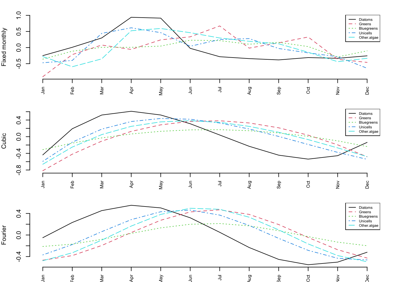
Estimated monthly effects for the three approaches to estimating seasonal effects. Top panel: each month modelled as a separate fixed effect for each taxon (60 parameters); Middle panel: monthly effects modelled as a 3rd order polynomial (20 parameters); Bottom panel: monthly effects modelled as a discrete Fourier series (10 parameters).

Figure 8.2: Estimated monthly effects for the three approaches to estimating seasonal effects. Top panel: each month modelled as a separate fixed effect for each taxon (60 parameters); Middle panel: monthly effects modelled as a 3rd order polynomial (20 parameters); Bottom panel: monthly effects modelled as a discrete Fourier series (10 parameters).

Rather than rely on our eyes to judge model fits, we should formally assess which of the 3 approaches offers the most parsimonious fit to the data. Here is a table of AICc values for the 3 models:

data.frame(Model = c("Fixed", "Cubic", "Fourier"), AICc = round(c(seas.mod.1$AICc, 
    seas.mod.2$AICc, seas.mod.3$AICc), 1))

    Model   AICc
1   Fixed 1188.4
2   Cubic 1144.9
3 Fourier 1127.4

The model selection results indicate that the model with monthly seasonal effects estimated via the discrete Fourier sequence is the best of the 3 models. Its AICc value is much lower than either the polynomial or fixed-effects models.