7.6 Using MARSS models to study spatial structure

For our next example, we will use MARSS models to test hypotheses about the population structure of harbor seals on the west coast. For this example, we will evaluate the support for different population structures (numbers of subpopulations) using different \(\mathbf{Z}\)s to specify how survey regions map onto subpopulations. We will assume correlated process errors with the same magnitude of process variance and covariance. We will assume independent observations errors with equal variances at each site. We could do unequal variances but it takes a long time to fit so for this example, the observation variances are set equal.

The dataset we will use is harborSeal, a 29-year dataset of abundance indices for 12 regions along the U.S. west coast between 1975-2004 (Figure 7.5).

We start by setting up our data matrix. We will leave off Hood Canal.

dat <- MARSS::harborSeal
years <- dat[, "Year"]
good <- !(colnames(dat) %in% c("Year", "HoodCanal"))
sealData <- t(dat[, good])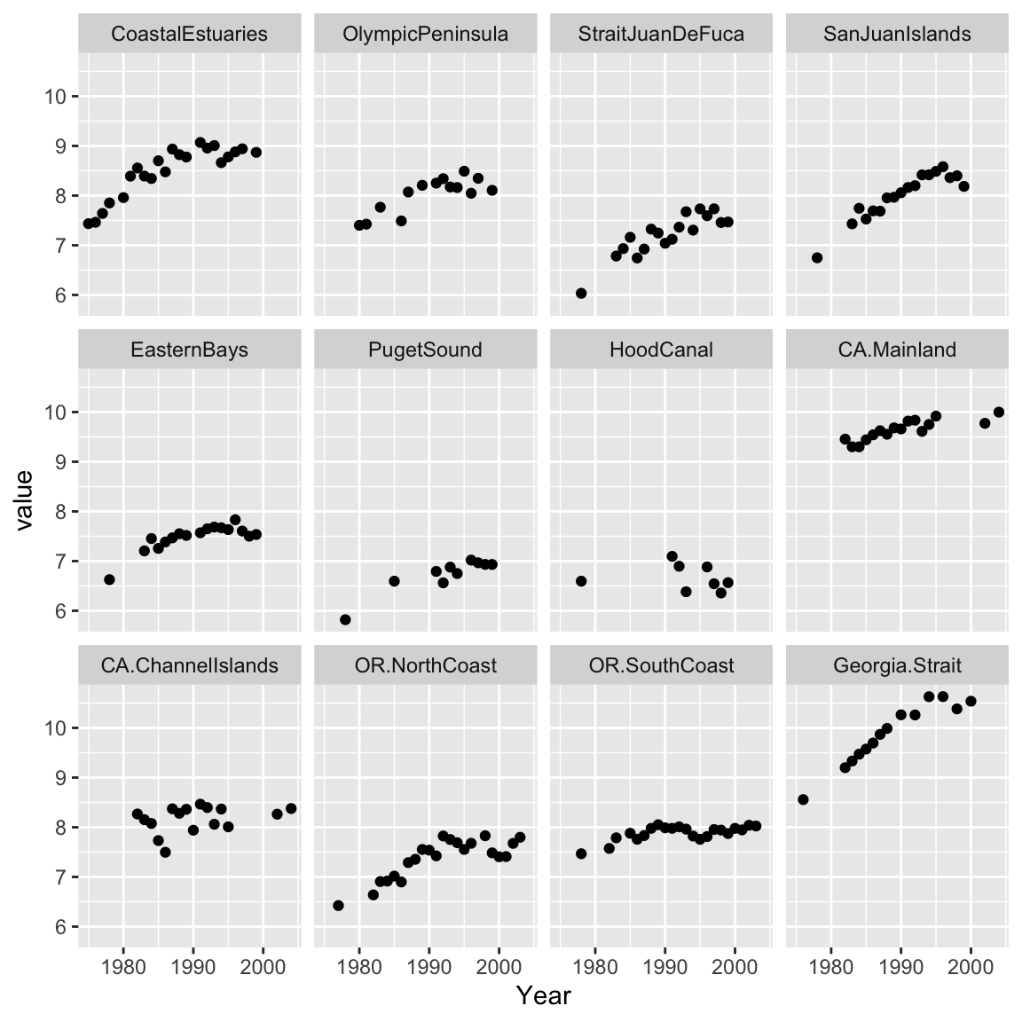

Figure 7.5: Plot of log counts at each survey region in the harborSeal dataset. Each region is an index of the harbor seal abundance in that region.