13.6 Dynamic factor analysis
First load the plankton dataset from the MARSS package.
library(MARSS)
data(lakeWAplankton, package = "MARSS")
# we want lakeWAplanktonTrans, which has been transformed
# so the 0s are replaced with NAs and the data z-scored
dat <- lakeWAplanktonTrans
# use only the 10 years from 1980-1989
plankdat <- dat[dat[, "Year"] >= 1980 & dat[, "Year"] < 1990,
    ]
# create vector of phytoplankton group names
phytoplankton <- c("Cryptomonas", "Diatoms", "Greens", "Unicells",
    "Other.algae")
# get only the phytoplankton
dat.spp.1980 <- t(plankdat[, phytoplankton])
# z-score the data since we subsetted time
dat.spp.1980 <- MARSS::zscore(dat.spp.1980)
# check our z-score
apply(dat.spp.1980, 1, mean, na.rm = TRUE)
Cryptomonas Diatoms Greens Unicells Other.algae
4.740855e-17 -5.592676e-18 -4.486354e-19 -2.699663e-18 6.517410e-18 apply(dat.spp.1980, 1, var, na.rm = TRUE)Cryptomonas Diatoms Greens Unicells Other.algae
1 1 1 1 1 Plot the data.
# make into ts since easier to plot
dat.ts <- ts(t(dat.spp.1980), frequency = 12, start = c(1980,
    1))
par(mfrow = c(3, 2), mar = c(2, 2, 2, 2))
for (i in 1:5) {
    plot(dat.ts[, i], type = "b", main = colnames(dat.ts)[i],
        col = "blue", pch = 16)
}
Figure 13.3: Phytoplankton data.
Run a 3 trend model on these data.
mod_3 <- bayesdfa::fit_dfa(y = dat.spp.1980, num_trends = 3,
    chains = 1, iter = 1000)
Rotate the estimated trends and look at what it produces.
rot <- bayesdfa::rotate_trends(mod_3)
names(rot)
[1] "Z_rot" "trends" "Z_rot_mean" "Z_rot_median"
[5] "trends_mean" "trends_median" "trends_lower" "trends_upper" Plot the estimate of the trends.
matplot(t(rot$trends_mean), type = "l", lwd = 2, ylab = "mean trend")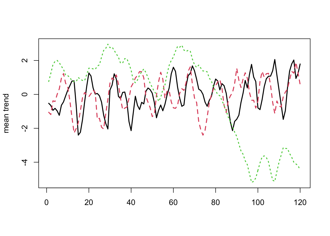
Figure 13.4: Trends.
13.6.1 Using leave one out cross-validation to select models
We will fit multiple DFA with different numbers of trends and use leave one out (LOO) cross-validation to choose the best model.
mod_1 <- bayesdfa::fit_dfa(y = dat.spp.1980, num_trends = 1,
    iter = 1000, chains = 1)
mod_2 <- bayesdfa::fit_dfa(y = dat.spp.1980, num_trends = 2,
    iter = 1000, chains = 1)
mod_3 <- bayesdfa::fit_dfa(y = dat.spp.1980, num_trends = 3,
    iter = 1000, chains = 1)
mod_4 <- bayesdfa::fit_dfa(y = dat.spp.1980, num_trends = 4,
    iter = 1000, chains = 1)
# mod_5 = bayesdfa::fit_dfa(y = dat.spp.1980, num_trends=5)
We will compute the Leave One Out Information Criterion (LOOIC) using the loo package. Like AIC, lower is better.
loo(mod_1)$estimates["looic", "Estimate"][1] 1613.758Table of the LOOIC values:
looics <- c(loo(mod_1)$estimates["looic", "Estimate"], loo(mod_2)$estimates["looic",
    "Estimate"], loo(mod_3)$estimates["looic", "Estimate"], loo(mod_4)$estimates["looic",
    "Estimate"])
looic.table <- data.frame(trends = 1:4, LOOIC = looics)
looic.table
trends LOOIC
1 1 1613.758
2 2 1540.511
3 3 1477.859
4 4 1457.230