4.6 Random walks (RW)

Random walks receive considerable attention in time series analyses because of their ability to fit a wide range of data despite their surprising simplicity. In fact, random walks are the most simple non-stationary time series model. A random walk is a time series \(\{x_t\}\) where

\[\begin{equation} \tag{4.18} x_t = x_{t-1} + w_t, \end{equation}\]

and \(w_t\) is a discrete white noise series where all values are independent and identically distributed (IID) with a mean of zero. In practice, we will almost always assume that the \(w_t\) are Gaussian white noise, such that \(w_t \sim \text{N}(0,q)\). We will see later that a random walk is a special case of an autoregressive model.

4.6.1 Simulating a random walk

Simulating a RW model in R is straightforward with a for loop and the use of rnorm() to generate Gaussian errors (type ?rnorm to see details on the function and its useful relatives dnorm() and pnorm()). Let’s create 100 obs (we’ll also set the random number seed so everyone gets the same results).

## set random number seed
set.seed(123)
## length of time series
TT <- 100
## initialize {x_t} and {w_t}
xx <- ww <- rnorm(n = TT, mean = 0, sd = 1)
## compute values 2 thru TT
for (t in 2:TT) {
    xx[t] <- xx[t - 1] + ww[t]
}

Now let’s plot the simulated time series and its ACF.

## setup plot area
par(mfrow = c(1, 2))
## plot line
plot.ts(xx, ylab = expression(italic(x[t])))
## plot ACF
plot.acf(acf(xx, plot = FALSE))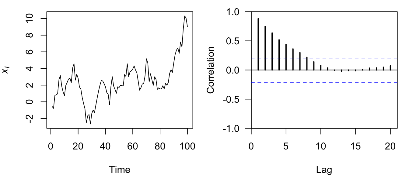

Figure 4.20: Simulated time series of a random walk model (left) and its associated ACF (right).

Perhaps not surprisingly based on their names, autoregressive models such as RW’s have a high degree of autocorrelation out to long lags (Figure 4.20).

4.6.2 Alternative formulation of a random walk

As an aside, let’s use an alternative formulation of a random walk model to see an even shorter way to simulate an RW in R. Based on our definition of a random walk in Equation (4.18), it is easy to see that

\[\begin{equation} \tag{4.19} \begin{aligned} x_t &= x_{t-1} + w_t \\ x_{t-1} &= x_{t-2} + w_{t-1} \\ x_{t-2} &= x_{t-3} + w_{t-2} \\ &\; \; \vdots \end{aligned} \end{equation}\]

Therefore, if we substitute \(x_{t-2} + w_{t-1}\) for \(x_{t-1}\) in the first equation, and then \(x_{t-3} + w_{t-2}\) for \(x_{t-2}\), and so on in a recursive manner, we get

\[\begin{equation} \tag{4.20} x_t = w_t + w_{t-1} + w_{t-2} + \dots + w_{t-\infty} + x_{t-\infty}. \end{equation}\]

In practice, however, the time series will not start an infinite time ago, but rather at some \(t=1\), in which case we can write

\[\begin{equation} \tag{4.21} \begin{aligned} x_t &= w_1 + w_2 + \dots + w_t \\ &= \sum_{t=1}^{T} w_t. \end{aligned} \end{equation}\]

From Equation (4.21) it is easy to see that the value of an RW process at time step \(t\) is the sum of all the random errors up through time \(t\). Therefore, in R we can easily simulate a realization from an RW process using the cumsum(x) function, which does cumulative summation of the vector x over its entire length. If we use the same errors as before, we should get the same results.

## simulate RW
x2 <- cumsum(ww)

Let’s plot both time series to see if it worked.

## setup plot area
par(mfrow = c(1, 2))
## plot 1st RW
plot.ts(xx, ylab = expression(italic(x[t])))
## plot 2nd RW
plot.ts(x2, ylab = expression(italic(x[t])))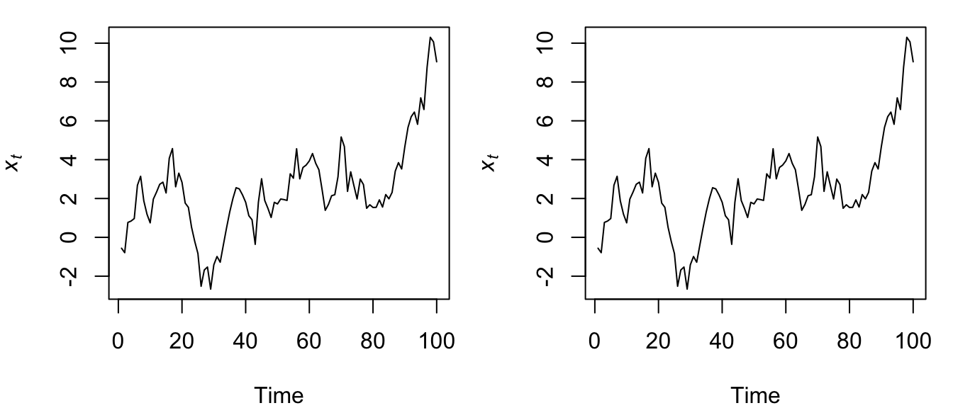

Figure 4.21: Time series of the same random walk model formulated as Equation (4.18) and simulated via a for loop (left), and as Equation (4.21) and simulated via cumsum() (right).

Indeed, both methods of generating a RW time series appear to be equivalent.