3.6 Classical decomposition

Model time series \(\{x_t\}\) as a combination of

trend (\(m_t\))
seasonal component (\(s_t\))
remainder (\(e_t\))

\(x_t = m_t + s_t + e_t\)

3.6.1 1. The trend (\(m_t\))

We need a way to extract the so-called signal. One common method is via “linear filters”

\[ m_t = \sum_{i=-\infty}^{\infty} \lambda_i x_{t+1} \]

For example, a moving average

\[ m_t = \sum_{i=-a}^{a} \frac{1}{2a + 1} x_{t+i} \]

If \(a = 1\), then

\[ m_t = \frac{1}{3}(x_{t-1} + x_t + x_{t+1}) \]

3.6.2 Example of linear filtering

Here is a time series.

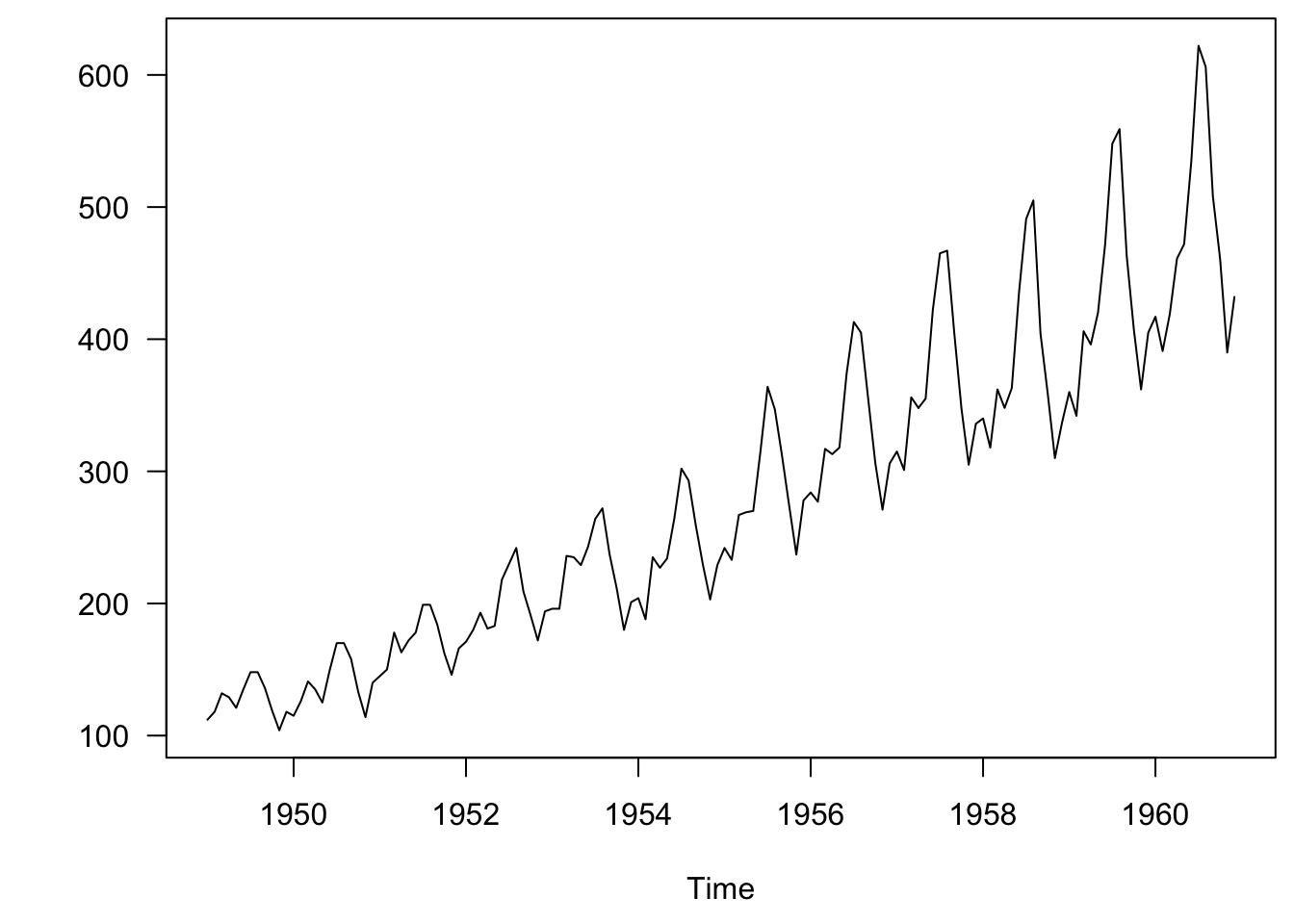
Figure 3.5: Monthly airline passengers from 1949-1960

A linear filter with \(a=3\) closely tracks the data.

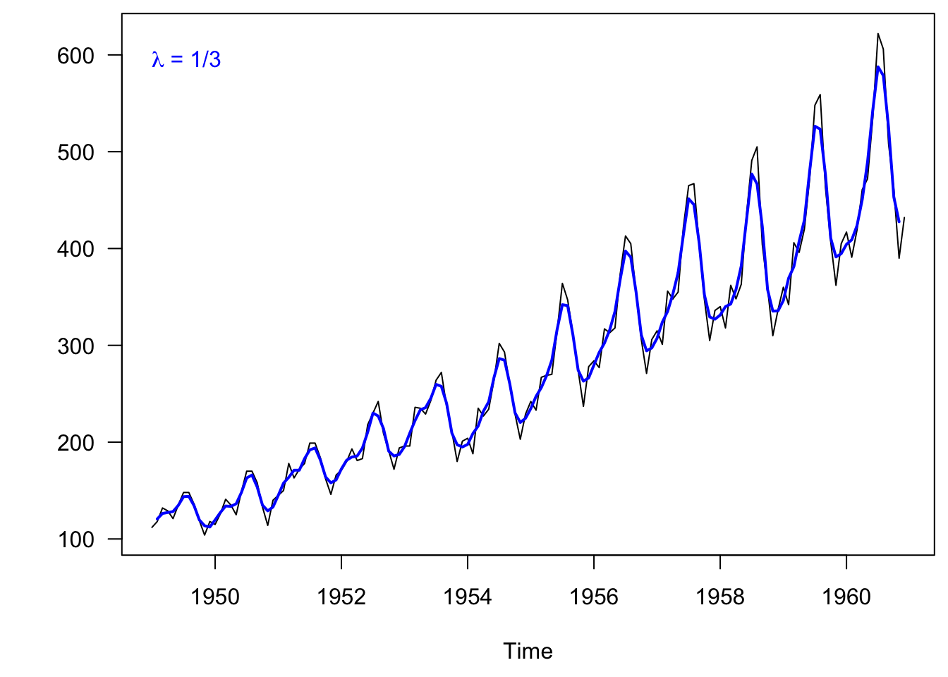
Figure 3.6: Monthly airline passengers from 1949-1960 with a low filter.

As we increase the length of data that is averaged from 1 on each side (\(a=3\)) to 4 on each side (\(a=9\)), the trend line is smoother.

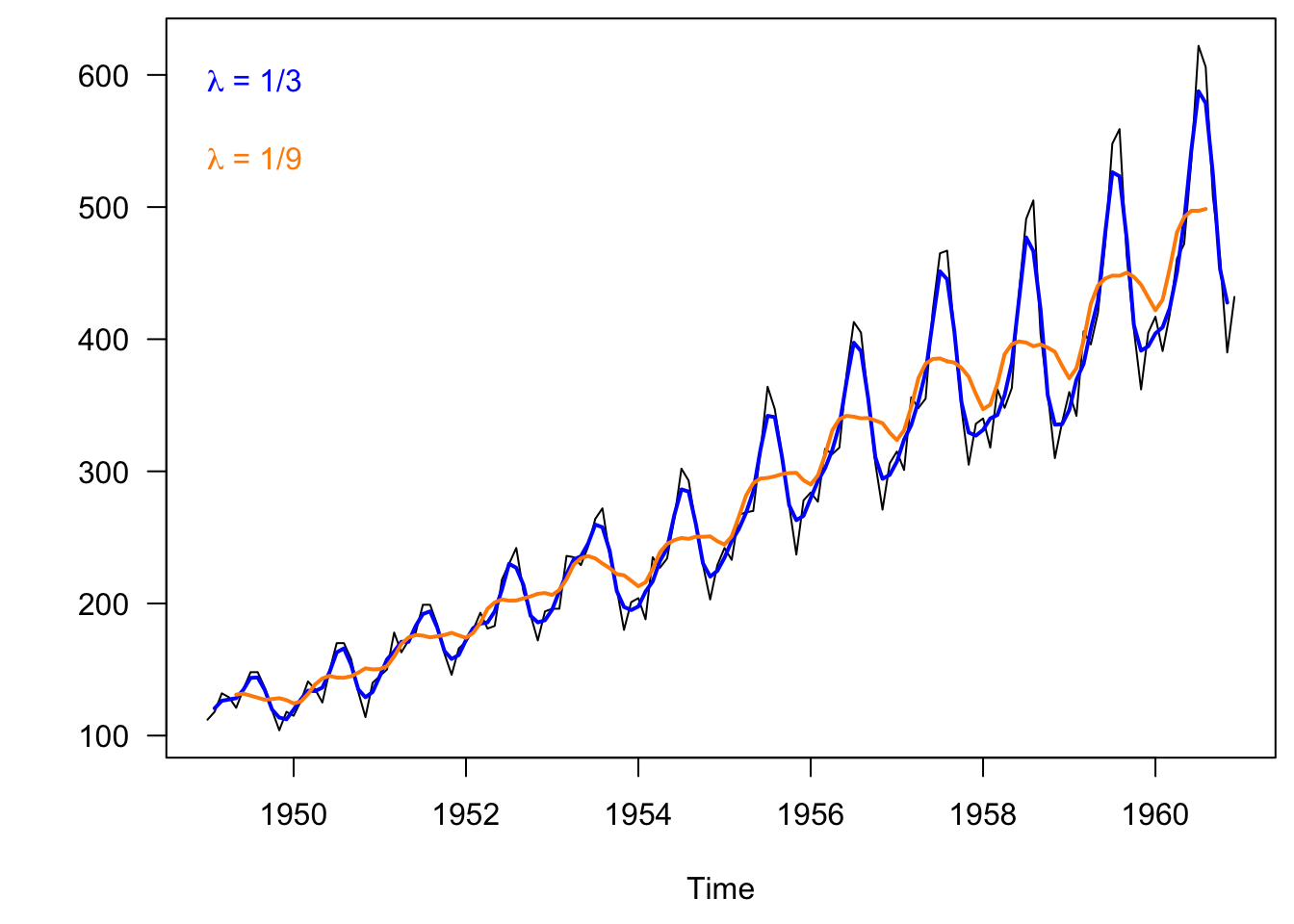
Figure 3.7: Monthly airline passengers from 1949-1960 with a medium filter.

When we increase up to 13 points on each side (\(a=27\)), the trend line is very smooth.

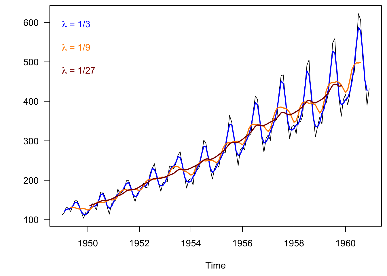
Figure 3.8: Monthly airline passengers from 1949-1960 with a high filter.

3.6.3 2. Seasonal effect (\(s_t\))

Once we have an estimate of the trend \(m_t\), we can estimate \(s_t\) simply by subtraction:

\[ s_t = x_t - m_t \]

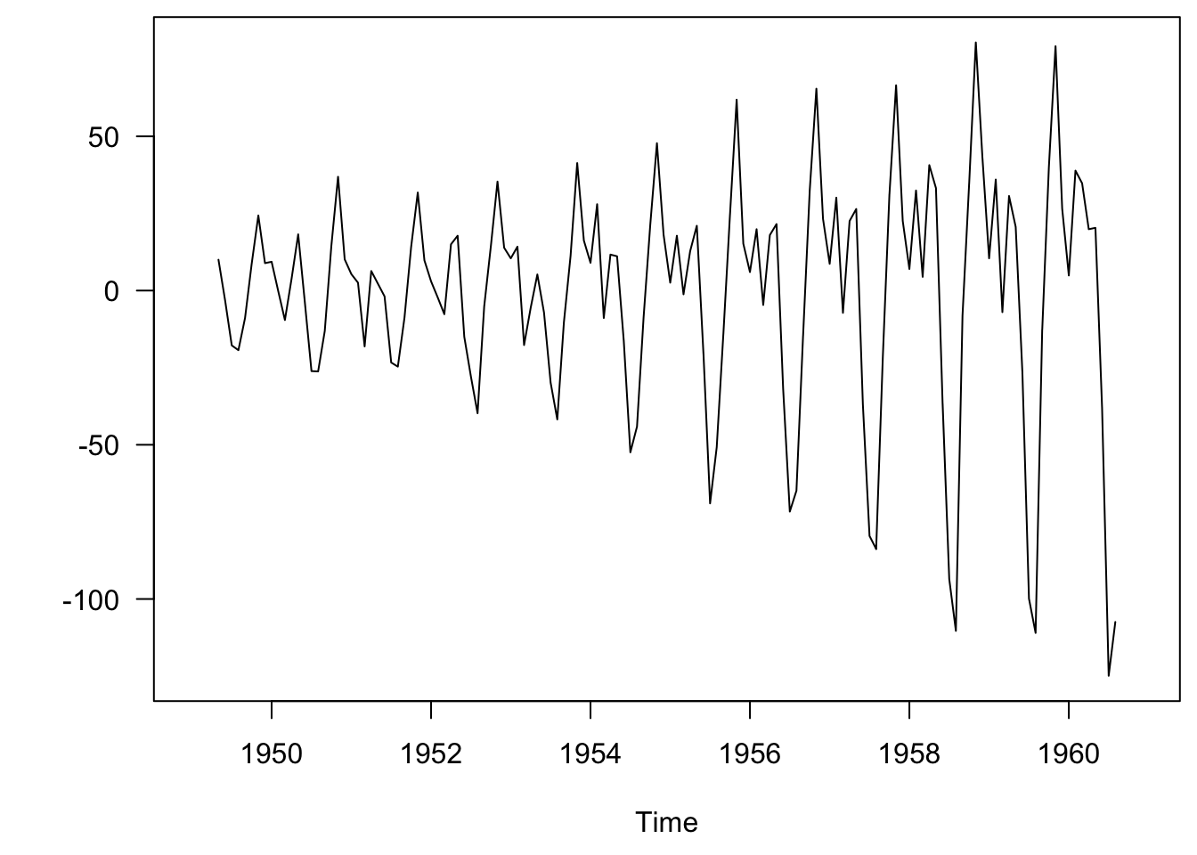
This is the seasonal effect (\(s_t\)), assuming \(\lambda = 1/9\), but, \(s_t\) includes the remainder \(e_t\) as well. Instead we can estimate the mean seasonal effect (\(s_t\)).

seas_2 <- decompose(xx)$seasonal
par(mai = c(0.9, 0.9, 0.1, 0.1), omi = c(0, 0, 0, 0))
plot.ts(seas_2, las = 1, ylab = "")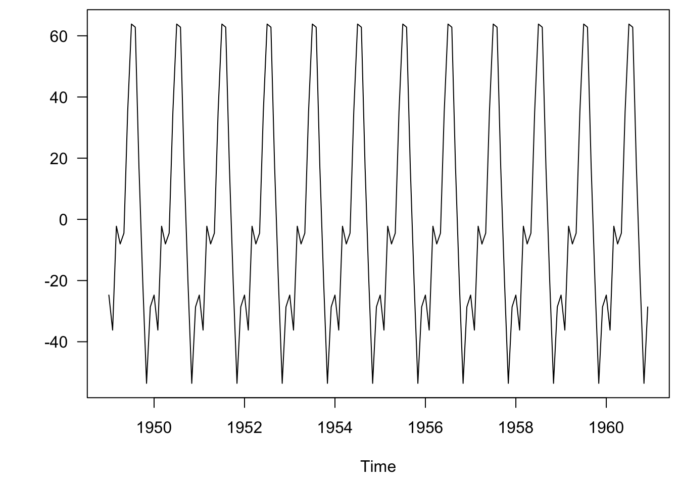

Figure 3.9: Mean seasonal effect.

3.6.4 3. Remainder (\(e_t\))

Now we can estimate \(e_t\) via subtraction:

\[ e_t = x_t - m_t - s_t \]

ee <- decompose(xx)$random
par(mai = c(0.9, 0.9, 0.1, 0.1), omi = c(0, 0, 0, 0))
plot.ts(ee, las = 1, ylab = "")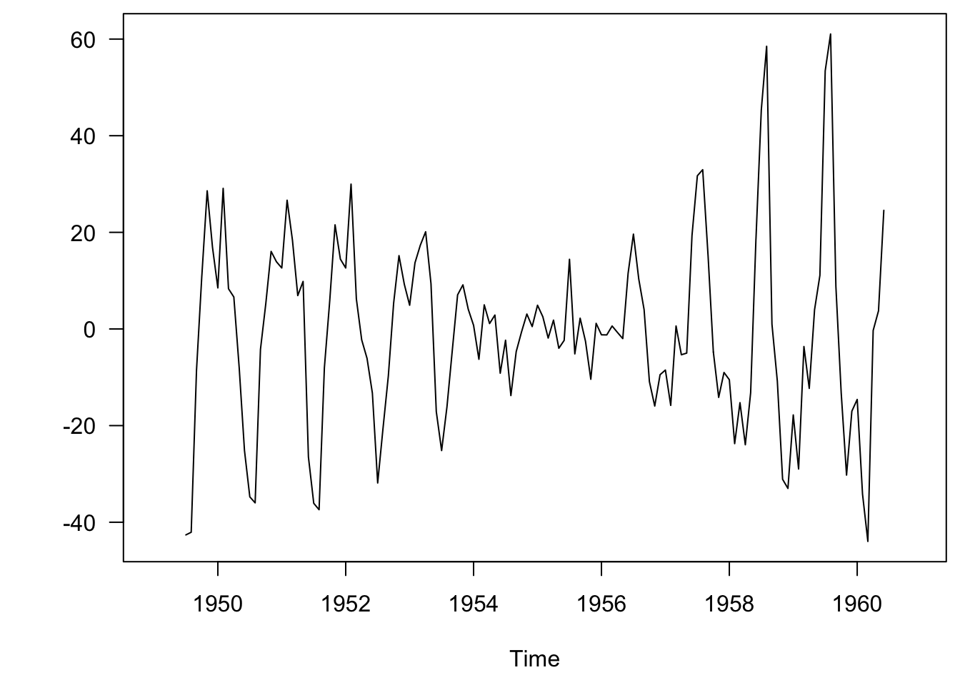

Figure 3.10: Errors.