6.5 Basic diagnostics
The first diagnostic that you do with any statistical analysis is check that your residuals correspond to your assumed error structure. For a basic residuals diagnostic check for a state-space model, we want to use the ‘innovations residuals.’ This is the observed data at time \(t\) minus the value predicted using the model plus the data up to time \(t-1\). Innovations residuals should be Gaussian and temporally independent (no autocorrelation).
residuals(fit) will return the innovations residuals as a data frame.
head(residuals(kem.0)) type .rownames name t value .fitted .resids .sigma .std.resids
1 ytt1 Y1 model 1871 1120 919.35 200.65 168.3792 1.1916552
2 ytt1 Y1 model 1872 1160 919.35 240.65 168.3792 1.4292142
3 ytt1 Y1 model 1873 963 919.35 43.65 168.3792 0.2592362
4 ytt1 Y1 model 1874 1210 919.35 290.65 168.3792 1.7261629
5 ytt1 Y1 model 1875 1160 919.35 240.65 168.3792 1.4292142
6 ytt1 Y1 model 1876 1160 919.35 240.65 168.3792 1.4292142The innovations residuals should also not be autocorrelated in time. We can check the autocorrelation with the function acf(). The autocorrelation plots are shown in Figure 6.3. The stochastic level model looks the best in that its innovations residuals are fine.
par(mfrow = c(2, 2), mar = c(2, 2, 4, 2))
resids <- residuals(kem.0)
acf(resids$.resids, main = "flat level v(t)", na.action = na.pass)
resids <- residuals(kem.1)
acf(resids$.resids, main = "linear trend v(t)", na.action = na.pass)
resids <- residuals(kem.2)
acf(resids$.resids, main = "stoc level v(t)", na.action = na.pass)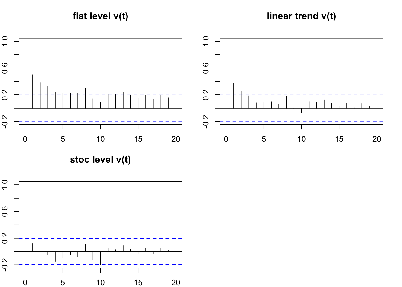
Figure 6.3: The model innovations residual acfs for the 3 models.
6.5.1 Outlier diagnostics
Another type of residual used in state-space models is smoothation residuals. This residual at time \(t\) is conditioned on all the data. Smoothation residuals are used for outlier detection and can help detect anomalous shocks in the data. Smoothation residuals can be autocorrelated but should fluctuate around 0. The should not have a trend. Looking at your smoothation residuals can help you determine if there are fundamental problems with the structure of your model.
We can get the smoothation residuals by passing in type="tT" to the residuals() call. Figure 6.4 shows the model and state smoothation residuals. The flat level and linear trend models do not have a stochastic state so their state residuals are all 0.
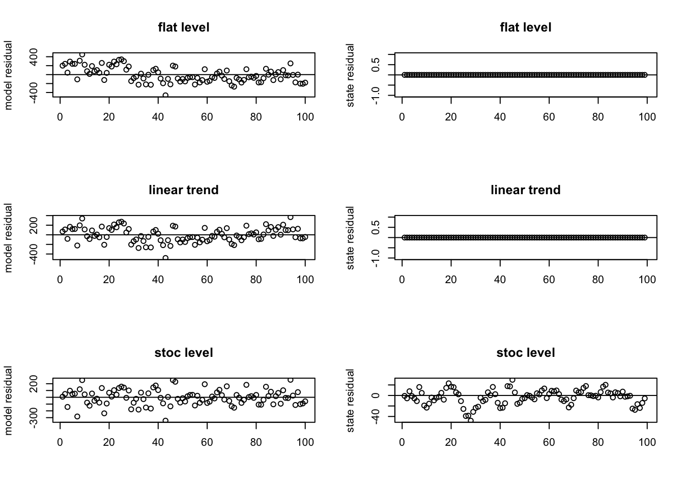
Figure 6.4: The model and state smoothations residuals for the first 3 models.
The flat and linear trend models show problems. The model smoothation residuals are positive early and then are slightly negative. They should fluctuate around 0 the whole time series. The stochastic level model looks fine. The residuals fluctuate around 0.
The smoothation residuals can also help us look for outliers in the data or outlier shifts in the level (sudden anolmalous changes). If we standardize by the variance of the residuals (divide by the square root of the variance), then the standardized residuals should have an approximate standard normal distribution.
We will look just at the stochastic level model since the other models do not have a stochastic state (\(x\)). Figure 6.5 (right panel) shows us that there was a sudden level change around 1902. The Aswan Low Dam was completed in 1902 and changed the mean flow. The Aswan High Dam was completed in 1970 and also affected the flow though not as much. You can see these perturbations in Figure 6.1.
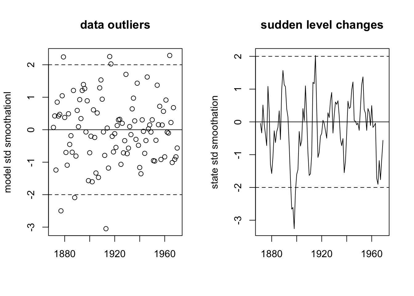
Figure 6.5: The model and state smoothations residuals for the first 3 models.