9.7 Fitting with MARSS()

Now let’s go ahead and analyze the DLM specified in Equations (9.19)–(9.21). We begin by loading the data set (which is in the MARSS package). The data set has 3 columns for 1) the year the salmon smolts migrated to the ocean (year), 2) logit-transformed survival (logit.s), and 3) the coastal upwelling index for April (CUI.apr). There are 42 years of data (1964–2005).

## load the data
data(SalmonSurvCUI, package = "MARSS")
## get time indices
years <- SalmonSurvCUI[, 1]
## number of years of data
TT <- length(years)
## get response variable: logit(survival)
dat <- matrix(SalmonSurvCUI[, 2], nrow = 1)

As we have seen in other case studies, standardizing our covariate(s) to have zero-mean and unit-variance can be helpful in model fitting and interpretation. In this case, it’s a good idea because the variance of CUI.apr is orders of magnitude greater than logit.s.

## get predictor variable
CUI <- SalmonSurvCUI[, 3]
## z-score the CUI
CUI_z <- matrix((CUI - mean(CUI))/sqrt(var(CUI)), nrow = 1)
## number of regr params (slope + intercept)
m <- dim(CUI_z)[1] + 1

Plots of logit-transformed survival and the \(z\)-scored April upwelling index are shown in Figure 9.1.

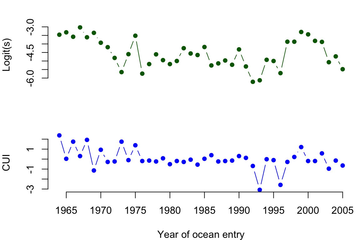
Figure 9.1: Time series of logit-transformed marine survival estimates for Snake River spring/summer Chinook salmon (top) and z-scores of the coastal upwelling index at 45N 125W (bottom). The x-axis indicates the year that the salmon smolts entered the ocean.

Next, we need to set up the appropriate matrices and vectors for MARSS. Let’s begin with those for the process equation because they are straightforward.

## for process eqn
B <- diag(m)  ## 2x2; Identity
U <- matrix(0, nrow = m, ncol = 1)  ## 2x1; both elements = 0
Q <- matrix(list(0), m, m)  ## 2x2; all 0 for now
diag(Q) <- c("q.alpha", "q.beta")  ## 2x2; diag = (q1,q2)

Defining the correct form for the observation model is a little more tricky, however, because of how we model the effect(s) of predictor variables. In a DLM, we need to use \(\mathbf{Z}_t\) (instead of \(\mathbf{d}_t\)) as the matrix of predictor variables that affect \(\mathbf{y}_t\), and we use \(\mathbf{x}_t\) (instead of \(\mathbf{D}_t\)) as the regression parameters. Therefore, we need to set \(\mathbf{Z}_t\) equal to an \(n\times m\times T\) array, where \(n\) is the number of response variables (= 1; \(y_t\) is univariate), \(m\) is the number of regression parameters (= intercept + slope = 2), and \(T\) is the length of the time series (= 42).

## for observation eqn
Z <- array(NA, c(1, m, TT))  ## NxMxT; empty for now
Z[1, 1, ] <- rep(1, TT)  ## Nx1; 1's for intercept
Z[1, 2, ] <- CUI_z  ## Nx1; predictor variable
A <- matrix(0)  ## 1x1; scalar = 0
R <- matrix("r")  ## 1x1; scalar = r

Lastly, we need to define our lists of initial starting values and model matrices/vectors.

## only need starting values for regr parameters
inits_list <- list(x0 = matrix(c(0, 0), nrow = m))

## list of model matrices & vectors
mod_list <- list(B = B, U = U, Q = Q, Z = Z, A = A, R = R)

And now we can fit our DLM with MARSS.

## fit univariate DLM
dlm_1 <- MARSS(dat, inits = inits_list, model = mod_list)

Success! abstol and log-log tests passed at 115 iterations.
Alert: conv.test.slope.tol is 0.5.
Test with smaller values (<0.1) to ensure convergence.

MARSS fit is
Estimation method: kem 
Convergence test: conv.test.slope.tol = 0.5, abstol = 0.001
Estimation converged in 115 iterations. 
Log-likelihood: -40.03813 
AIC: 90.07627   AICc: 91.74293   
 
          Estimate
R.r        0.15708
Q.q.alpha  0.11264
Q.q.beta   0.00564
x0.X1     -3.34023
x0.X2     -0.05388
Initial states (x0) defined at t=0

Standard errors have not been calculated. 
Use MARSSparamCIs to compute CIs and bias estimates.

Notice that the MARSS output does not list any estimates of the regression parameters themselves. Why not? Remember that in a DLM the matrix of states \((\mathbf{x})\) contains the estimates of the regression parameters \((\boldsymbol{\theta})\). Therefore, we need to look in dlm_1$states for the MLEs of the regression parameters, and in dlm_1$states.se for their standard errors.

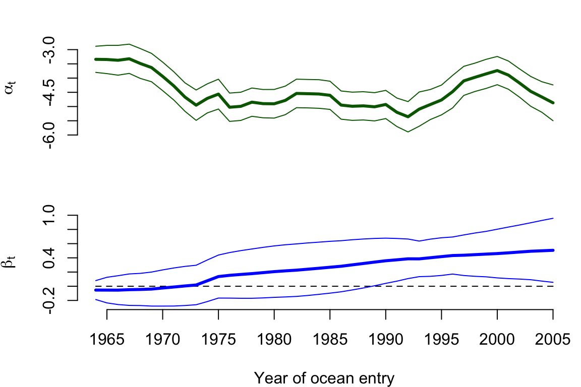
Time series of the estimated intercept and slope are shown in Figure 9.2. It appears as though the intercept is much more dynamic than the slope, as indicated by a much larger estimate of process variance for the former (Q.q1). In fact, although the effect of April upwelling appears to be increasing over time, it doesn’t really become important as a predictor variable until about 1990 when the approximate 95% confidence interval for the slope no longer overlaps zero.

Figure 9.2: Time series of estimated mean states (thick lines) for the intercept (top) and slope (bottom) parameters from the DLM specified by Equations (9.19)–(9.21). Thin lines denote the mean \(\pm\) 2 standard deviations.