7.3 A single well-mixed population
When we are looking at data over a large geographic region, we might make the assumption that the different census regions are measuring a single population if we think animals are moving sufficiently such that the whole area (multiple regions together) is “well-mixed.” We write a model of the total population abundance for this case as: \[\begin{equation} n_t = \,\text{exp}(u + w_t) n_{t-1}, \tag{7.2} \end{equation}\] where \(n_t\) is the total count in year \(t\), \(u\) is the mean population growth rate, and \(w_t\) is the deviation from that average in year \(t\). We then take the log of both sides and write the model in log space: \[\begin{equation} x_t = x_{t-1} + u + w_t, \textrm{ where } w_t \sim \,\text{N}(0,q) \tag{7.3} \end{equation}\] \(x_t=\log{n_t}\). When there is one effective population, there is one \(x\), therefore \(\mathbf{x}_t\) is a \(1 \times 1\) matrix. This is our state model and \(x\) is called the “state.” This is just the jargon used in this type of model (state-space model) for the hidden state that you are estimating from the data. “Hidden” means that you observe this state with error.
7.3.1 The observation process
We assume that all four regional time series are observations of this one population trajectory but they are scaled up or down relative to that trajectory. In effect, we think of each regional survey as an index of the total population. With this model, we do not think the regions represent independent subpopulations but rather independent observations of one population. Our model for the data, \(\mathbf{y}_t = \mathbf{Z} \mathbf{x}_t + \mathbf{a} + \mathbf{v}_t\), is written as: \[\begin{equation} \left[ \begin{array}{c} y_{1} \\ y_{2} \\ y_{3} \\ y_{4} \end{array} \right]_t = \left[ \begin{array}{c} 1\\ 1\\ 1\\ 1\end{array} \right] x_t + \left[ \begin{array}{c} 0 \\ a_2 \\ a_3 \\ a_4 \end{array} \right] + \left[ \begin{array}{c} v_{1} \\ v_{2} \\ v_{3} \\ v_{4} \end{array} \right]_t \tag{7.4} \end{equation}\] Each \(y_{i}\) is the observed time series of counts for a different region. The \(a\)’s are the bias between the regional sample and the total population. \(\mathbf{Z}\) specifies which observation time series, \(y_i\), is associated with which population trajectory, \(x_j\). In this case, \(\mathbf{Z}\) is a matrix with 1 column since each region is an observation of the one population trajectory.
We allow that each region could have a unique observation variance and that the observation errors are independent between regions. We assume that the observations errors on log(counts) are normal and thus the errors on (counts) are log-normal. The assumption of normality is not unreasonable since these regional counts are the sum of counts across multiple haul-outs. We specify independent observation errors with different variances by specifying that \(\mathbf{v} \sim \,\text{MVN}(0,\mathbf{R})\), where
\[\begin{equation}
\mathbf{R} = \begin{bmatrix}
r_1 & 0 & 0 & 0 \\
0 & r_2 & 0 & 0\\
0 & 0 & r_3 & 0 \\
0 & 0 & 0 & r_4 \end{bmatrix}
\tag{7.5}
\end{equation}\]
This is a diagonal matrix with unequal variances. The shortcut for this structure in MARSS() is "diagonal and unequal".
7.3.2 Fitting the model
We need to write the model in the form of Equation (7.1) with each parameter written as a matrix. The observation model (Equation (7.4)) is already in matrix form. Let’s write the state model in matrix form too: \[\begin{equation} [x]_t = [1][x]_{t-1} + [u] + [w]_t, \textrm{ where } [w]_t \sim \,\text{N}(0,[q]) \tag{7.6} \end{equation}\] It is very simple since all terms are \(1 \times 1\) matrices.
To fit our model with MARSS(), we set up a list which precisely describes the size and structure of each parameter matrix. Fixed values in a matrix are designated with their numeric value and estimated values are given a character name and put in quotes. Our model list for a single well-mixed population is:
mod.list.0 <- list(B = matrix(1), U = matrix("u"), Q = matrix("q"),
    Z = matrix(1, 4, 1), A = "scaling", R = "diagonal and unequal",
    x0 = matrix("mu"), tinitx = 0)
and fit:
fit.0 <- MARSS(dat, model = mod.list.0)Success! abstol and log-log tests passed at 32 iterations.
Alert: conv.test.slope.tol is 0.5.
Test with smaller values (<0.1) to ensure convergence.
MARSS fit is
Estimation method: kem
Convergence test: conv.test.slope.tol = 0.5, abstol = 0.001
Estimation converged in 32 iterations.
Log-likelihood: 21.62931
AIC: -23.25863 AICc: -19.02786
Estimate
A.SJI 0.79583
A.EBays 0.27528
A.PSnd -0.54335
R.(SJF,SJF) 0.02883
R.(SJI,SJI) 0.03063
R.(EBays,EBays) 0.01661
R.(PSnd,PSnd) 0.01168
U.u 0.05537
Q.q 0.00642
x0.mu 6.22810
Initial states (x0) defined at t=0
Standard errors have not been calculated.
Use MARSSparamCIs to compute CIs and bias estimates.We already discussed that the short-cut "diagonal and unequal" means a diagonal matrix with each diagonal element having a different value. The short-cut "scaling" means the form of \(\mathbf{a}\) in Equation (7.4) with one value set to 0 and the rest estimated. You should run the code in the list to make sure you see that each parameter in the list has the same form as in our mathematical equation for the model.
7.3.3 Model residuals
The model fits fine but look at the model residuals (Figure 7.2). They have problems.
par(mfrow = c(2, 2))
resids <- MARSSresiduals(fit.0, type = "tt1")
for (i in 1:4) {
    plot(resids$model.residuals[i, ], ylab = "model residuals",
        xlab = "")
    abline(h = 0)
    title(rownames(dat)[i])
}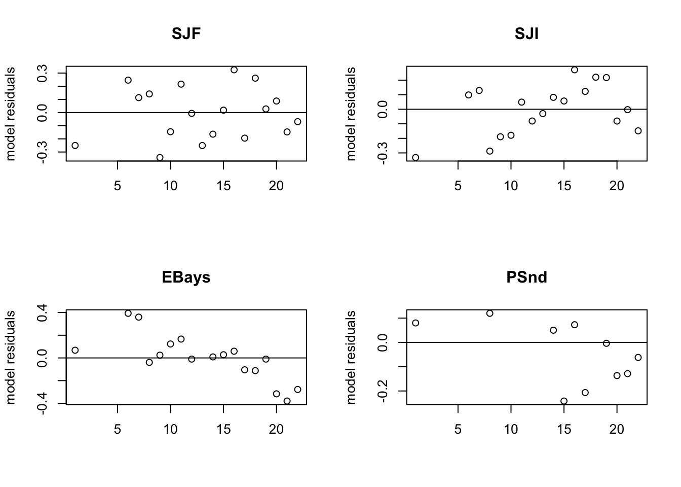
Figure 7.2: The model residuals for the first model. SJI and EBays do not look good.