7.11 Problems

For these questions, use the harborSealWA data set in MARSS. The data are already logged, but you will need to remove the year column and have time going across the columns not down the rows.

require(MARSS)
data(harborSealWA, package = "MARSS")
dat <- t(harborSealWA[, 2:6])

The sites are San Juan de Fuca (SJF 3), San Juan Islands (SJI 4), Eastern Bays (EBays 5), Puget Sound (PSnd 6) and Hood Canal (HC 7).

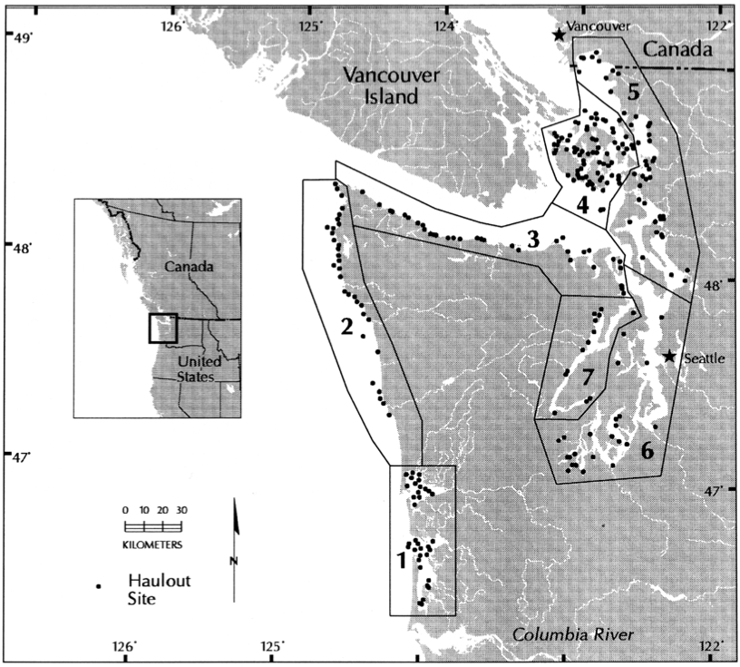
Regions in the harbor seal surveys

Plot the harbor seal data. Use whatever plotting functions you wish (e.g. ggplot(), plot(); points(); lines(), matplot()).
Fit a panmictic population model that assumes that each of the 5 sites is observing one “Inland WA” harbor seal population with trend $u$. Assume the observation errors are independent and identical. This means 1 variance on diagonal and 0s on off-diagonal. This is the default assumption for MARSS().
1. Write the $\mathbf{Z}$ for this model. The code to use for making a matrix in Rmarkdown is
```
$$\begin{bmatrix}a & b & 0\\d & e & f\\0 & h & i\end{bmatrix}$$
```
1. Write the $\mathbf{Z}$ matrix in R using Z=matrix(...) and using the factor short-cut for specifying $\mathbf{Z}$. Z=factor(c(...).
2. Fit the model using MARSS(). What is the estimated trend ($u$)? How fast was the population increasing (percent per year) based on this estimated $u$?
3. Compute the confidence intervals for the parameter estimates. Compare the intervals using the Hessian approximation and using a parametric bootstrap. What differences do you see between the two approaches? Use this code:
```
library(broom)
tidy(fit)
# set nboot low so it doesn't take forever
tidy(fit, method="parametric",nboot=100)
```
1. What does an estimate of $\mathbf{Q}=0$ mean? What would the estimated state ($x$) look like when $\mathbf{Q}=0$?
Using the same panmictic population model, compare 3 assumptions about the observation error structure.
- The observation errors are independent with different variances.
- The observation errors are independent with the same variance.
- The observation errors are correlated with the same variance and same correlation.
1. Write the $\mathbf{R}$ variance-covariance matrices for each assumption.
2. Create each R matrix in R. To combine, numbers and characters in a matrix use a list matrix like so:
```
A <- matrix(list(0),3,3)
A[1,1] <- "sigma2"
```
1. Fit each model using MARSS() and compute the confidence intervals (CIs) for the estimated parameters. Compare the estimated $u$ (the population long-term trend) along with their CIs. Does the assumption about the observation errors change the $u$ estimate?
2. Plot the state residuals, the ACF of the state residuals, and the histogram of the state residuals for each fit. Are there any issues that you see? Use this code to get your state residuals:
```
MARSSresiduals(fit)$state.residuals[1,]
```
You need the [1,] since the residuals are returned as a matrix.
Fit a model with 3 subpopulations. 1=SJF,SJI; 2=PS,EBays; 3=HC. The $x$ part of the model is the population structure. Assume that the observation errors are identical and independent (R="diagonal and equal"). Assume that the process errors are unique and independent (Q="diagonal and unequal"). Assume that the $u$ are unique among the 3 subpopulation.
1. Write the $\mathbf{x}$ equation. Make sure each matrix in the equation has the right number of rows and columns.
2. Write the $\mathbf{Z}$ matrix.
3. Write the $\mathbf{Z}$ in R using Z=matrix(...) and using the factor shortcut Z=factor(c(...)).
4. Fit the model with MARSS().
5. What do the estimated $u$ and $\mathbf{Q}$ imply about the population dynamics in the 3 subpopulations?
Repeat the fit from Question 4 but assume that the 3 subpopulations covary. Use Q="unconstrained".
1. What does the estimated $\mathbf{Q}$ matrix tell you about how the 3 subpopulation covary?
2. Compare the AICc from the model in Question 4 and the one with Q="unconstrained". Which is more supported?
3. Fit the model with Q="equalvarcov". Is this more supported based on AICc?
Develop the following alternative models for the structure of the inland harbor seal population. For each model assume that the observation errors are identical and independent (R="diagonal and equal"). Assume that the process errors covary with equal variance and covariances (Q="equalvarcov").
- 5 subpopulations with unique $u$.
- 5 subpopulations with shared (equal) $u$.
- 5 subpopulations but with $u$ shared in some regions: SJF+SJI shared, PS+EBays shared, HC unique.
- 1 panmictic population.
- 3 subpopulations, 1=SJF,SJI, 2=PS,EBays, 3=HC, with unique $u$
- 2 subpopulations, 1=SJF,SJI,PS,EBays, 2=HC, with unique $u$
1. Fit each model using MARSS().
2. Prepare a table of each model with a column for the AICc values. And a column for $\Delta AICc$ (AICc minus the lowest AICc in the group). What is the most supported model?
Do diagnostics on the model innovations residuals for the 3 subpopulation model from question 4. Use the following code to get your model residuals. This will put NAs in the model residuals where there is missing data. Then do the tests on each row of resids.
```
resids <- MARSSresiduals(fit, type = "tt1")$model.residuals
resids[is.na(dat)] <- NA
```
1. Plot the model residuals.
2. Plot the ACF of the model residuals. Use acf(..., na.action=na.pass).
3. Plot the histogram of the model residuals.
4. Fit an ARIMA() model to your model residuals using forecast::auto.arima(). Are the best fit models what you want? Note, we cannot use the Augmented Dickey-Fuller or KPSS tests when there are missing values in our residuals time series.