8.7 Model diagnostics

We will examine some basic model diagnostics for these three approaches by looking at plots of the model residuals and their autocorrelation functions (ACFs) for all five taxa using the following code:

for (i in 1:3) {
    dev.new()
    modn <- paste("seas.mod", i, sep = ".")
    for (j in 1:5) {
        resid.j <- MARSSresiduals(get(modn), type = "tt1")$model.residuals[j, 
            ]
        plot.ts(resid.j, ylab = "Residual", main = phytos[j])
        abline(h = 0, lty = "dashed")
        acf(resid.j, na.action = na.pass)
    }
}

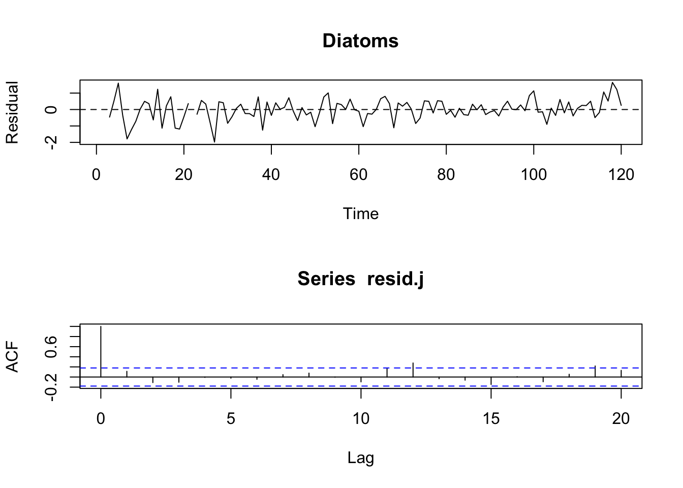
Figure 8.3: Residuals for model with season modelled as a discrete Fourier series.