12.3 Multivariate state-space models
In the multivariate state-space model, our observations and hidden states can be multivariate along with all the parameters: \[\begin{equation} \begin{gathered} \mathbf{x}_t = \mathbf{B} \mathbf{x}_{t-1}+\mathbf{u}+\mathbf{w}_t \text{ where } \mathbf{w}_t \sim \,\text{N}(0,\mathbf{Q}) \\ \mathbf{y}_t = \mathbf{Z}\mathbf{x}_t+\mathbf{a}+\mathbf{v}_t \text{ where } \mathbf{v}_t \sim \,\text{N}(0,\mathbf{R}) \\ \mathbf{x}_0 = \boldsymbol{\mu} \end{gathered} \tag{12.9} \end{equation}\]
12.3.1 One hidden state
Let’s start with a very simple MARSS model with JAGS: two observation time-series and one hidden state. Our \(\mathbf{x}_t\) model is \(x_t = x_{t-1} + u + w_t\) and our \(\mathbf{y}_t\) model is \[\begin{equation} \begin{bmatrix} y_{1} \\ y_{2}\end{bmatrix}_t = \begin{bmatrix} 1\\ 1\end{bmatrix} x_t + \begin{bmatrix} 0 \\ a_2\end{bmatrix} + \begin{bmatrix} v_{1} \\ v_{2}\end{bmatrix}_t, \, \begin{bmatrix} v_{1} \\ v_{2}\end{bmatrix}_t \sim \,\text{MVN}\left(0, \begin{bmatrix} r_1&0 \\ 0&r_2\end{bmatrix}\right) \tag{12.10} \end{equation}\]
We need to put a prior on our \(x_0\) (initial \(x\)). Since \(b=1\), we have a random walk rather than a stationary process and we will put a vague prior on the \(x_0\). We need to deal with the \(\mathbf{a}\) so that our code doesn’t run in circles by trying to match \(x\) up with different \(y_t\) time series. We force \(x_t\) to track the mean of \(y_{1,t}\) and then use \(a_2\) to scale the other \(y_t\) relative to that. The problem is that a random walk is very flexible and if we tried to estimate \(a_1\) then we would have infinite solutions.
To keep our JAGS code organized, let’s separate the \(\mathbf{x}\) and \(\mathbf{y}\) parts of the code.
jagsscript <- cat("
model {
   # process model priors
   u ~ dnorm(0, 0.01); # one u
   inv.q~dgamma(0.001,0.001);
   q <- 1/inv.q; # one q
   X0 ~ dnorm(Y1,0.001); # initial state
   # process model likelihood
   EX[1] <- X0 + u;
   X[1] ~ dnorm(EX[1], inv.q);
   for(t in 2:N) {
         EX[t] <- X[t-1] + u;
         X[t] ~ dnorm(EX[t], inv.q);
   }

   # observation model priors
   for(i in 1:n) { # r's differ by site
     inv.r[i]~dgamma(0.001,0.001);
     r[i] <- 1/inv.r[i];
   }
   a[1] <- 0; # first a is 0, rest estimated
   for(i in 2:n) {
     a[i]~dnorm(0,0.001);
   }
   # observation model likelihood
   for(t in 1:N) {
     for(i in 1:n) {
       EY[i,t] <- X[t]+a[i]
       Y[i,t] ~ dnorm(EY[i,t], inv.r[i]);
     }
   }
}

",
    file = "marss-jags1.txt")
To fit the model, we write the data list, parameter list, and pass the model to the jags() function.
data(harborSealWA, package = "MARSS")
dat <- t(harborSealWA[, 2:3])
jags.data <- list(Y = dat, n = nrow(dat), N = ncol(dat), Y1 = dat[1,
    1])
jags.params <- c("EY", "u", "q", "r")
model.loc <- "marss-jags1.txt"  # name of the txt file
mod_marss1 <- R2jags::jags(jags.data, parameters.to.save = jags.params,
    model.file = model.loc, n.chains = 3, n.burnin = 5000, n.thin = 1,
    n.iter = 10000, DIC = TRUE)
We can make a plot of our estimated parameters:
post.params <- mod_marss1$BUGSoutput$sims.list
par(mfrow = c(2, 2))
hist(log(post.params$q), main = "log(q)", xlab = "")
hist(post.params$u, main = "u", xlab = "")
hist(log(post.params$r[, 1]), main = "log(r_1)", xlab = "")
hist(log(post.params$r[, 2]), main = "log(r_2)", xlab = "")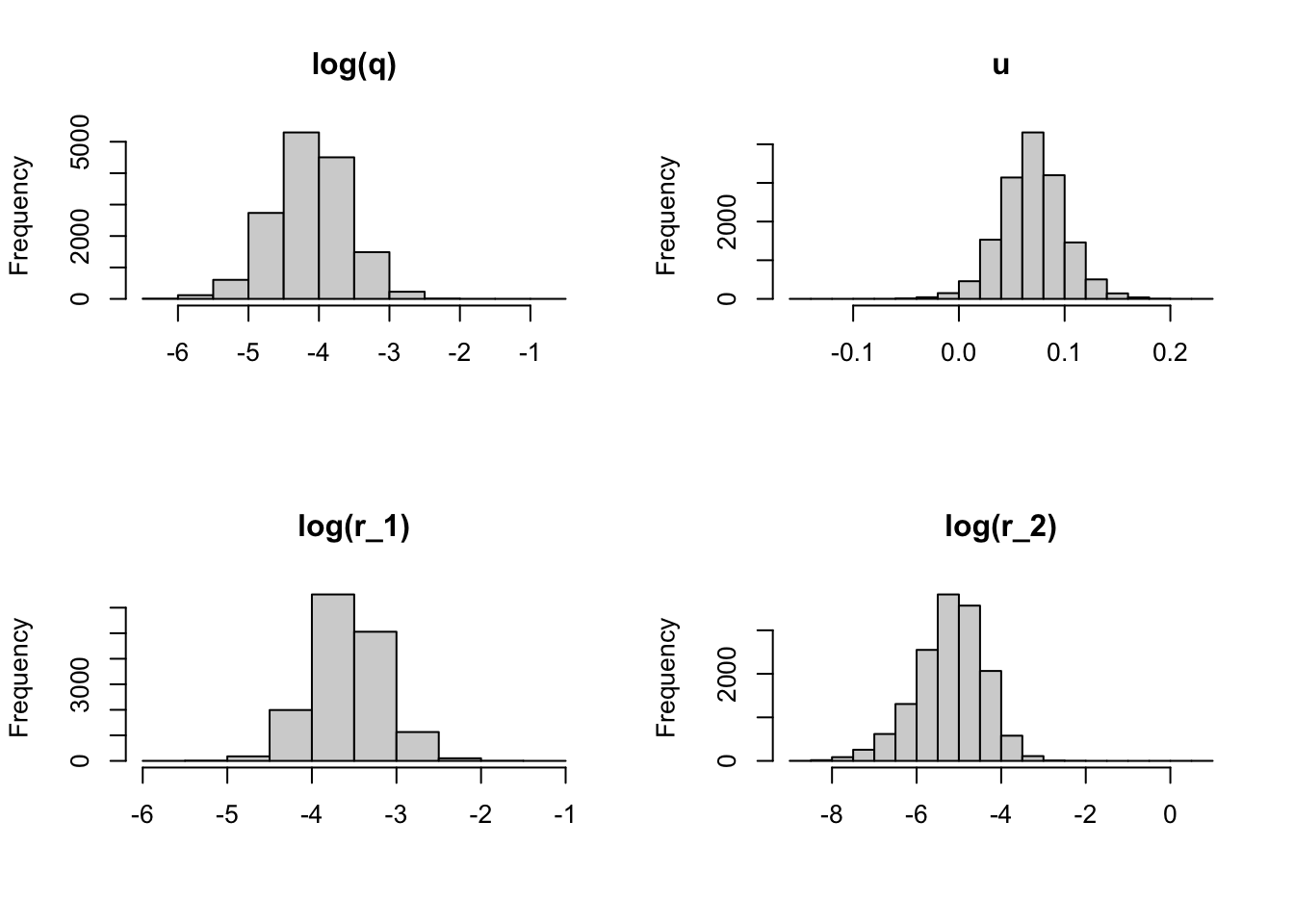
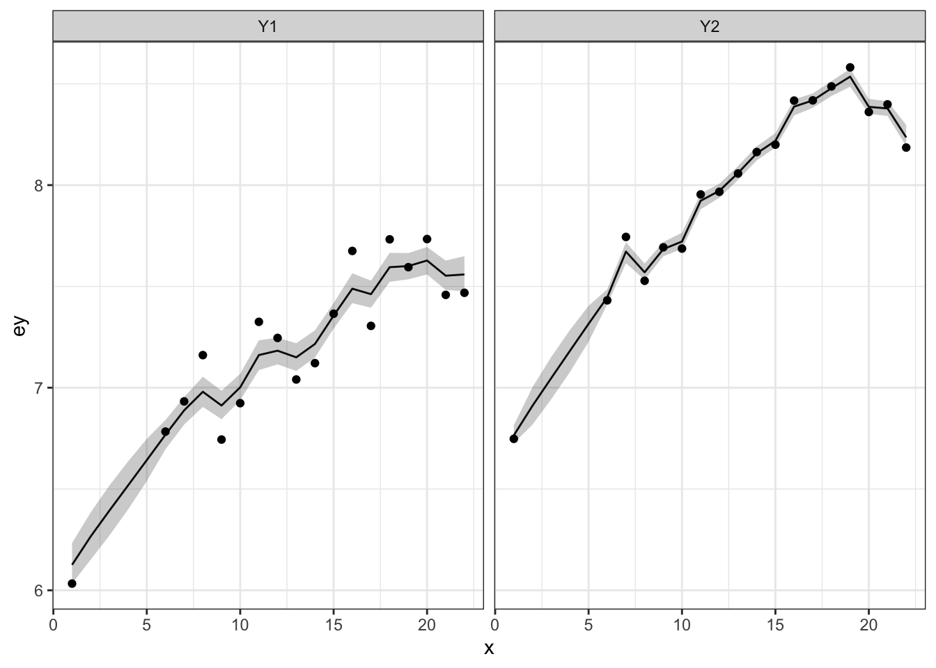
We can make a plot of the model fitted \(y_t\) with 50% credible intervals and the data. Note that the credible intervals are for the expected value of \(y_{i,t}\) so will be narrower than the data.
make.ey.plot <- function(mod, dat) {
    library(ggplot2)
    EY <- mod$BUGSoutput$sims.list$EY
    n <- nrow(dat)
    N <- ncol(dat)
    df <- c()
    for (i in 1:n) {
        tmp <- data.frame(n = paste0("Y", i), x = 1:N, ey = apply(EY[,
            i, , drop = FALSE], 3, median), ey.low = apply(EY[,
            i, , drop = FALSE], 3, quantile, probs = 0.25), ey.up = apply(EY[,
            i, , drop = FALSE], 3, quantile, probs = 0.75), y = dat[i,
            ])
        df <- rbind(df, tmp)
    }
    ggplot(df, aes(x = x, y = ey)) + geom_line() + geom_ribbon(aes(ymin = ey.low,
        ymax = ey.up), alpha = 0.25) + geom_point(data = df,
        aes(x = x, y = y)) + facet_wrap(~n) + theme_bw()
}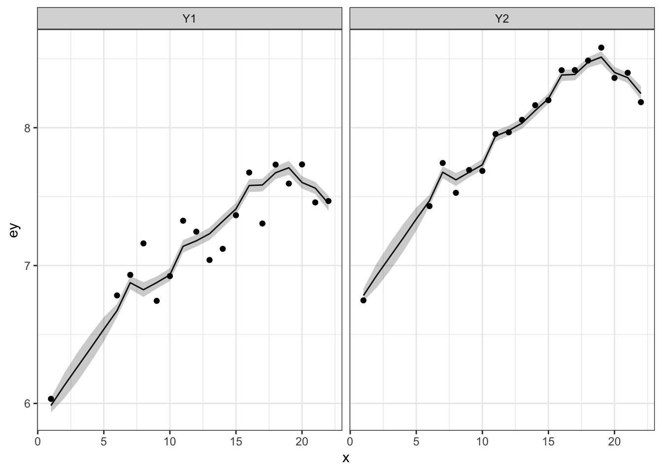
12.3.2 \(m\) hidden states
Let’s add multiple hidden states. We’ll say that each \(y_t\) is observing its own \(x_t\) but the \(x_t\) share the same \(q\) but not \(u\). Our \(\mathbf{x}_t\) model is \[\begin{equation} \begin{bmatrix} x_{1} \\ x_{2}\end{bmatrix}_t = \begin{bmatrix} 1&0\\ 0&1\end{bmatrix} \begin{bmatrix} x_{1} \\ x_{2}\end{bmatrix}_{t-1} + \begin{bmatrix} u_1 \\ u_2\end{bmatrix} + \begin{bmatrix} w_{1} \\ w_{2}\end{bmatrix}_t, \, \begin{bmatrix} w_{1} \\ w_{2}\end{bmatrix}_t \sim \,\text{MVN}\left(0, \begin{bmatrix} q&0 \\ 0&q\end{bmatrix}\right) (\#eq:jags-marss2) \end{equation}\]
Here is the JAGS model. Note that \(a_i\) is 0 for all \(i\) because each \(y_t\) is associated with its own \(x_t\).
jagsscript <- cat("
model {
   # process model priors
   inv.q~dgamma(0.001,0.001);
   q <- 1/inv.q; # one q
   for(i in 1:n) {
      u[i] ~ dnorm(0, 0.01);
      X0[i] ~ dnorm(Y1[i],0.001); # initial states
   }
   # process model likelihood
   for(i in 1:n) {
     EX[i,1] <- X0[i] + u[i];
     X[i,1] ~ dnorm(EX[i,1], inv.q);
   }
   for(t in 2:N) {
      for(i in 1:n) {
         EX[i,t] <- X[i,t-1] + u[i];
         X[i,t] ~ dnorm(EX[i,t], inv.q);
      }
   }

   # observation model priors
   for(i in 1:n) { # The r's are different by site
     inv.r[i]~dgamma(0.001,0.001);
     r[i] <- 1/inv.r[i];
   }
   # observation model likelihood
   for(t in 1:N) {
     for(i in 1:n) {
       EY[i,t] <- X[i,t]
       Y[i,t] ~ dnorm(EY[i,t], inv.r[i]);
     }
   }
}

",
    file = "marss-jags2.txt")
Our code to fit the model changes a little.
data(harborSealWA, package = "MARSS")
dat <- t(harborSealWA[, 2:3])
jags.data <- list(Y = dat, n = nrow(dat), N = ncol(dat), Y1 = dat[,
    1])
jags.params <- c("EY", "u", "q", "r")
model.loc <- "marss-jags2.txt"  # name of the txt file
mod_marss1 <- R2jags::jags(jags.data, parameters.to.save = jags.params,
    model.file = model.loc, n.chains = 3, n.burnin = 5000, n.thin = 1,
    n.iter = 10000, DIC = TRUE)