9.8 Forecasting

Forecasting from a DLM involves two steps:

1. Get an estimate of the regression parameters at time \(t\) from data up to time \(t-1\). These are also called the one-step ahead forecast (or prediction) of the regression parameters.

2. Make a prediction of \(y\) at time \(t\) based on the predictor variables at time \(t\) and the estimate of the regression parameters at time \(t\) (step 1). This is also called the one-step ahead forecast (or prediction) of the observation.

9.8.1 Estimate of the regression parameters

For step 1, we want to compute the distribution of the regression parameters at time \(t\) conditioned on the data up to time \(t-1\), also known as the one-step ahead forecasts of the regression parameters. Let’s denote \(\boldsymbol{\theta}_{t-1}\) conditioned on \(y_{1:t-1}\) as \(\boldsymbol{\theta}_{t-1|t-1}\) and denote \(\boldsymbol{\theta}_{t}\) conditioned on \(y_{1:t-1}\) as \(\boldsymbol{\theta}_{t|t-1}\). We will start by defining the distribution of \(\boldsymbol{\theta}_{t|t}\) as follows

\[\begin{equation} \tag{9.23} \boldsymbol{\theta}_{t|t} \sim \text{MVN}(\boldsymbol{\pi}_t,\boldsymbol{\Lambda}_t) \end{equation}\] where \(\boldsymbol{\pi}_t = \text{E}(\boldsymbol{\theta}_{t|t})\) and \(\mathbf{\Lambda}_t = \text{Var}(\boldsymbol{\theta}_{t|t})\).

Now we can compute the distribution of \(\boldsymbol{\theta}_{t}\) conditioned on \(y_{1:t-1}\) using the process equation for \(\boldsymbol{\theta}\):

\[\begin{equation} \boldsymbol{\theta}_{t} = \mathbf{G}_t \boldsymbol{\theta}_{t-1} + \mathbf{w}_t, \, \mathbf{w}_t \sim \text{MVN}(\mathbf{0}, \mathbf{Q}) \end{equation}\]

The expected value of \(\boldsymbol{\theta}_{t|t-1}\) is thus

\[\begin{equation} \tag{9.24} \text{E}(\boldsymbol{\theta}_{t|t-1}) = \mathbf{G}_t \text{E}(\boldsymbol{\theta}_{t-1|t-1}) = \mathbf{G}_t \boldsymbol{\pi}_{t-1} \end{equation}\]

The variance of \(\boldsymbol{\theta}_{t|t-1}\) is

\[\begin{equation} \tag{9.25} \text{Var}(\boldsymbol{\theta}_{t|t-1}) = \mathbf{G}_t \text{Var}(\boldsymbol{\theta}_{t-1|t-1}) \mathbf{G}_t^{\top} + \mathbf{Q} = \mathbf{G}_t \mathbf{\Lambda}_{t-1} \mathbf{G}_t^{\top} + \mathbf{Q} \end{equation}\]

Thus the distribution of \(\boldsymbol{\theta}_{t}\) conditioned on \(y_{1:t-1}\) is

\[\begin{equation} \tag{9.26} \text{E}(\boldsymbol{\theta}_{t|t-1}) \sim \text{MVN}(\mathbf{G}_t \boldsymbol{\pi}_{t-1}, \mathbf{G}_t \mathbf{\Lambda}_{t-1} \mathbf{G}_t^{\top} + \mathbf{Q}) \end{equation}\]

9.8.2 Prediction of the response variable \(y_t\)

For step 2, we make the prediction of \(y_{t}\) given the predictor variables at time \(t\) and the estimate of the regression parameters at time \(t\). This is called the one-step ahead prediction for the observation at time \(t\). We will denote the prediction of \(y\) as \(\hat{y}\) and we want to compute its distribution (mean and variance). We do this using the equation for \(y_t\) but substituting the expected value of \(\boldsymbol{\theta}_{t|t-1}\) for \(\boldsymbol{\theta}_t\).

\[\begin{equation} \tag{9.27} \hat{y}_{t|t-1} = \mathbf{F}^{\top}_{t} \text{E}(\boldsymbol{\theta}_{t|t-1}) + e_{t}, \, e_{t} \sim \text{N}(0, r) \end{equation}\]

Our prediction of \(y\) at \(t\) has a normal distribution with mean (expected value) and variance. The expected value of \(\hat{y}_{t|t-1}\) is

\[\begin{equation} \tag{9.28} \text{E}(\hat{y}_{t|t-1}) = \mathbf{F}^{\top}_{t} \text{E}(\boldsymbol{\theta}_{t|t-1}) = \mathbf{F}^{\top}_{t} (\mathbf{G}_t \boldsymbol{\pi}_{t-1}) \end{equation}\]

and the variance of \(\hat{y}_{t|t-1}\) is

\[\begin{align} \tag{9.29} \text{Var}(\hat{y}_{t|t-1}) &= \mathbf{F}^{\top}_{t} \text{Var}(\boldsymbol{\theta}_{t|t-1}) \mathbf{F}_{t} + r \\ &= \mathbf{F}^{\top}_{t} (\mathbf{G}_t \mathbf{\Lambda}_{t-1} \mathbf{G}_t^{\top} + \mathbf{Q}) \mathbf{F}_{t} + r \end{align}\]

9.8.3 Computing the prediction

The expectations and variance of \(\boldsymbol{\theta}_t\) conditioned on \(y_{1:t}\) and \(y_{1:t-1}\) are standard output from the Kalman filter. Thus to produce the predictions, all we need to do is run our DLM state-space model through a Kalman filter to get \(\text{E}(\boldsymbol{\theta}_{t|t-1})\) and \(\text{Var}(\boldsymbol{\theta}_{t|t-1})\) and then use Equation (9.28) to compute the mean prediction and Equation (9.29) to compute its variance.

The Kalman filter will need \(\mathbf{F}_t\), \(\mathbf{G}_t\) and estimates of \(\mathbf{Q}\) and \(r\). The latter are calculated by fitting the DLM to the data \(y_{1:t}\), using for example the MARSS() function.

Let’s see an example with the salmon survival DLM. We will use the Kalman filter function in the MARSS package and the DLM fit from MARSS().

9.8.4 Forecasting salmon survival

Scheuerell and Williams (2005) were interested in how well upwelling could be used to actually forecast expected survival of salmon, so let’s look at how well our model does in that context. To do so, we need the predictive distribution for the survival at time \(t\) given the upwelling at time \(t\) and the predicted regression parameters at \(t\).

In the salmon survival DLM, the \(\mathbf{G}_t\) matrix is the identity matrix, thus the mean and variance of the one-step ahead predictive distribution for the observation at time \(t\) reduces to (from Equations (9.28) and (9.29))

\[\begin{equation} \begin{gathered} \tag{9.30} \text{E}(\hat{y}_{t|t-1}) = \mathbf{F}^{\top}_{t} \text{E}(\boldsymbol{\theta}_{t|t-1}) \\ \text{Var}(\hat{y}_{t|t-1}) = \mathbf{F}^{\top}_{t} \text{Var}(\boldsymbol{\theta}_{t|t-1}) \mathbf{F}_{t} + \hat{r} \end{gathered} \end{equation}\]

where

\[ \mathbf{F}_{t}=\begin{bmatrix}1 \\ f_{t}\end{bmatrix} \]

and \(f_{t}\) is the upwelling index at \(t+1\). \(\hat{r}\) is the estimated observation variance from our model fit.

9.8.5 Forecasting using MARSS

Working from Equation (9.30), we can compute the expected value of the forecast at time \(t\) and its variance using the Kalman filter. For the expectation, we need \(\mathbf{F}_{t}^\top\text{E}(\boldsymbol{\theta}_{t|t-1})\). \(\mathbf{F}_t^\top\) is called \(\mathbf{Z}_t\) in MARSS notation. The one-step ahead forecasts of the regression parameters at time \(t\), the \(\text{E}(\boldsymbol{\theta}_{t|t-1})\), are calculated as part of the Kalman filter algorithm—they are termed \(\tilde{x}_t^{t-1}\) in MARSS notation and stored as xtt1 in the list produced by the MARSSkfss() Kalman filter function.

Using the Z defined in 9.6, we compute the mean forecast as follows:

## get list of Kalman filter output
kf_out <- MARSSkfss(dlm_1)

## forecasts of regr parameters; 2xT matrix
eta <- kf_out$xtt1

## ts of E(forecasts)
fore_mean <- vector()
for (t in 1:TT) {
    fore_mean[t] <- Z[, , t] %*% eta[, t, drop = FALSE]
}

For the variance of the forecasts, we need \(\mathbf{F}^{\top}_{t} \text{Var}(\boldsymbol{\theta}_{t|t-1}) \mathbf{F}_{t} + \hat{r}\). As with the mean, \(\mathbf{F}^\top_t \equiv \mathbf{Z}_t\). The variances of the one-step ahead forecasts of the regression parameters at time \(t\), \(\text{Var}(\boldsymbol{\theta}_{t|t-1})\), are also calculated as part of the Kalman filter algorithm—they are stored as Vtt1 in the list produced by the MARSSkfss() function. Lastly, the observation variance \(\hat{r}\) was estimated when we fit the DLM to the data using MARSS() and can be extracted from the dlm_1 fit.

Putting this together, we can compute the forecast variance:

## variance of regr parameters; 1x2xT array
Phi <- kf_out$Vtt1

## obs variance; 1x1 matrix
R_est <- coef(dlm_1, type = "matrix")$R

## ts of Var(forecasts)
fore_var <- vector()
for (t in 1:TT) {
    tZ <- matrix(Z[, , t], m, 1)  ## transpose of Z
    fore_var[t] <- Z[, , t] %*% Phi[, , t] %*% tZ + R_est
}

Plots of the model mean forecasts with their estimated uncertainty are shown in Figure 9.3. Nearly all of the observed values fell within the approximate prediction interval. Notice that we have a forecasted value for the first year of the time series (1964), which may seem at odds with our notion of forecasting at time \(t\) based on data available only through time \(t-1\). In this case, however, MARSS is actually estimating the states at \(t=0\) (\(\boldsymbol{\theta}_0\)), which allows us to compute a forecast for the first time point.

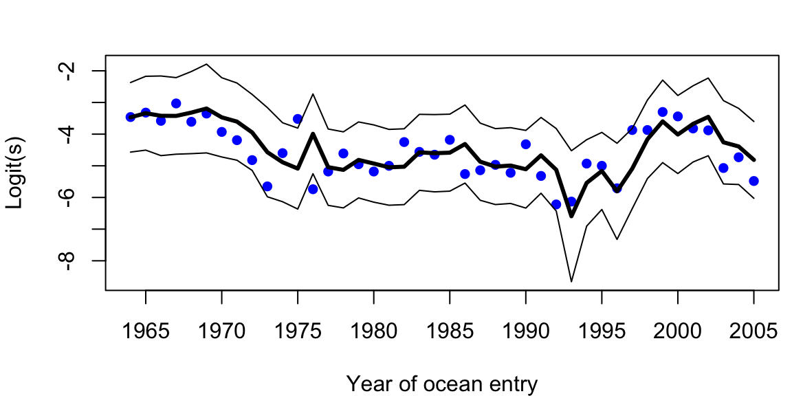
Figure 9.3: Time series of logit-transformed survival data (blue dots) and model mean forecasts (thick line). Thin lines denote the approximate 95% prediction intervals.

Although our model forecasts look reasonable in logit-space, it is worthwhile to examine how well they look when the survival data and forecasts are back-transformed onto the interval [0,1] (Figure 9.4). In that case, the accuracy does not seem to be affected, but the precision appears much worse, especially during the early and late portions of the time series when survival is changing rapidly.

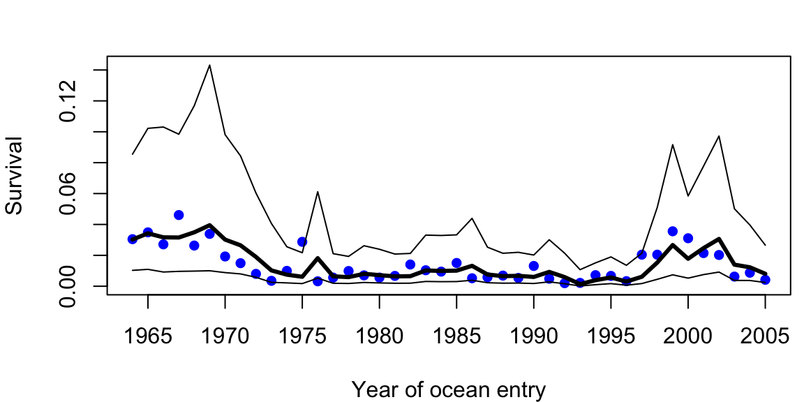
Figure 9.4: Time series of survival data (blue dots) and model mean forecasts (thick line). Thin lines denote the approximate 95% prediction intervals.

Notice that we passed the DLM fit to all the data to MARSSkfss(). This meant that the Kalman filter used estimates of \(\mathbf{Q}\) and \(r\) using all the data in the xtt1 and Vtt1 calculations. Thus our predictions at time \(t\) are not entirely based on only data up to time \(t-1\) since the \(\mathbf{Q}\) and \(r\) estimates were from all the data from 1964 to 2005.