12.2 Univariatate response models
12.2.1 Linear regression with no covariates
We will start with a linear regression with only an intercept. We will write the model in the form of Equation (12.1). Our model is \[\begin{equation} \begin{gathered} x_t = u \\ y_t = x_t + v_t, v_t \sim \,\text{N}(0, r) \end{gathered} \tag{12.2} \end{equation}\] An equivalent way to think about this model is \[\begin{equation} Y_t \sim \,\text{N}(E[Y_t], r) \end{equation}\] \(E[Y_{t}] = x_t\) where \(x_t = u\). In this linear regression model, we will treat the residual error as independent and identically distributed Gaussian observation error.
To run the JAGS model, we will need to start by writing the model in JAGS notation. We can construct the model in Equation (12.2) as
# LINEAR REGRESSION intercept only.

model.loc <- "lm_intercept.txt"  # name of the txt file
jagsscript <- cat("
model {
   # priors on parameters
   u ~ dnorm(0, 0.01);
   inv.r ~ dgamma(0.001,0.001); # This is inverse gamma
   r <- 1/inv.r; # derived value

   # likelihood
   for(i in 1:N) {
      X[i] <- u
      EY[i] <- X[i]; # derived value
      Y[i] ~ dnorm(EY[i], inv.r);
   }
}
",
    file = model.loc)
The JAGS code has three parts: our parameter priors, our data model and derived parameters.
Parameter priors There are two parameters in the model (\(u\), the mean, and \(r\), the variance of the observation error). We need to set a prior on both of these. We will set a vague prior of a Gaussian with varianc 10 on \(u\). In JAGS instead of specifying the normal distribution with the variance, \(N(0, 10)\), you specify it with the precision (1/variance), so our prior on \(u\) is dnorm(0, 0.01). For \(r\), we need to set a prior on the precision \(1/r\), which we call inv.r in the code. The precision receives a gamma prior, which is equivalent to the variance receiving an inverse gamma prior (fairly common for standard Bayesian regression models).
Likelihood Our data distribution is \(Y_t \sim \,\text{N}(E[Y_t], r)\). We use the dnorm() distribution with the precision (\(1/r\)) instead of \(r\). So our data model is Y[t] = dnorm(EY[t], inv.r). JAGS is not vectorized so we need to use for loops (instead of matrix multiplication) and use the for loop to specify the distribution for each Y[t]. For, this model we didn’t actually need X[t] but we use it because we are building up to a state-space model which has both \(x_t\) and \(y_t\).
Derived values Derived values are things we want output so we can track them. In this example, our derived values are a bit useless but in more complex models they will be quite handy. Also they can make your code easier to understand.
To run the model, we need to create several new objects, representing (1) a list of data that we will pass to JAGS jags.data, (2) a vector of parameters that we want to monitor and have returned back to R jags.params, and (3) the name of our text file that contains the JAGS model we wrote above. With those three things, we can call the jags() function.
jags.data <- list(Y = Wind, N = N)
jags.params <- c("r", "u")  # parameters to be monitored
mod_lm_intercept <- R2jags::jags(jags.data, parameters.to.save = jags.params,
    model.file = model.loc, n.chains = 3, n.burnin = 5000, n.thin = 1,
    n.iter = 10000, DIC = TRUE)
The function from the R2jags package that we use to run the model is jags(). There is a parallel version of the function called jags.parallel() which is useful for larger, more complex models. The details of both can be found with ?jags or ?jags.parallel.
Notice that the jags() function contains a number of other important arguments. In general, larger is better for all arguments: we want to run multiple MCMC chains (maybe 3 or more), and have a burn-in of at least 5000. The total number of samples after the burn-in period is n.iter-n.burnin, which in this case is 5000 samples. Because we are doing this with 3 MCMC chains, and the thinning rate equals 1 (meaning we are saving every sample), we will retain a total of 1500 posterior samples for each parameter.
The saved object storing our model diagnostics can be accessed directly, and includes some useful summary output.
mod_lm_interceptInference for Bugs model at "lm_intercept.txt", fit using jags,
3 chains, each with 10000 iterations (first 5000 discarded)
n.sims = 15000 iterations saved
mu.vect sd.vect 2.5% 25% 50% 75% 97.5% Rhat n.eff
r 12.563 1.469 10.009 11.525 12.460 13.484 15.752 1.001 15000
u 9.950 0.287 9.378 9.757 9.950 10.145 10.502 1.001 15000
deviance 820.566 2.013 818.591 819.137 819.943 821.342 826.073 1.001 15000
For each parameter, n.eff is a crude measure of effective sample size,
and Rhat is the potential scale reduction factor (at convergence, Rhat=1).
DIC info (using the rule, pD = var(deviance)/2)
pD = 2.0 and DIC = 822.6
DIC is an estimate of expected predictive error (lower deviance is better).The last two columns in the summary contain Rhat (which we want to be close to 1.0), and neff (the effective sample size of each set of posterior draws). To examine the output more closely, we can pull all of the results directly into R,
R2jags::attach.jags(mod_lm_intercept)Attaching the R2jags object loads the posteriors for the parameters and we can call them directly, e.g. u. If we don’t want to attach them to our workspace, we can find the posteriors within the model object.
post.params <- mod_lm_intercept$BUGSoutput$sims.listWe make a histogram of the posterior distributions of the parameters u and r with the following code,
# Now we can make plots of posterior values
par(mfrow = c(2, 1))
hist(post.params$u, 40, col = "grey", xlab = "u", main = "")
hist(post.params$r, 40, col = "grey", xlab = "r", main = "")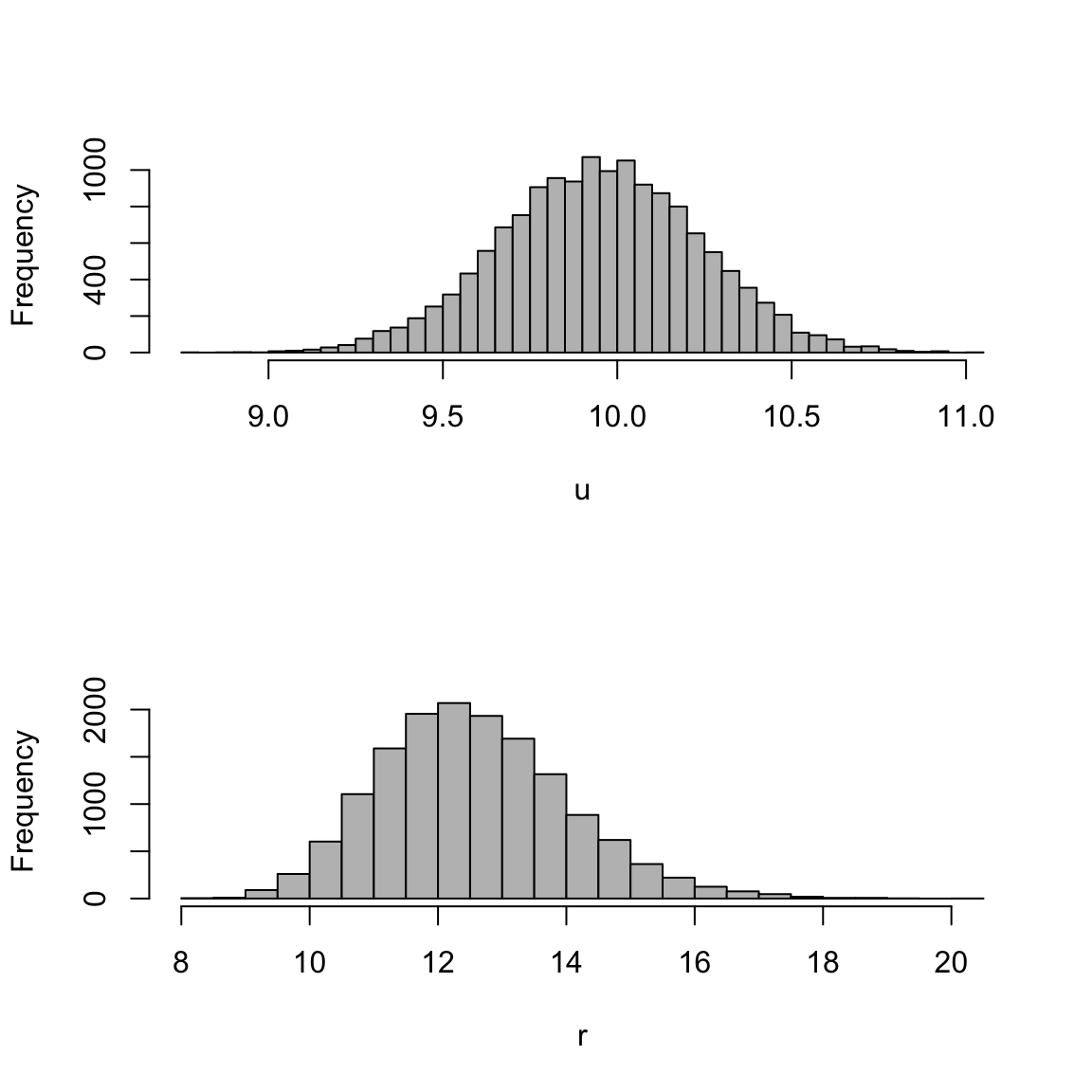
Figure 12.1: Plot of the posteriors for the linear regression model.
We can run some useful diagnostics from the coda package on this model output. We have written a small function to make the creation of a MCMC list (an argument required for many of the diagnostics). The function is
createMcmcList <- function(jagsmodel) {
    McmcArray <- as.array(jagsmodel$BUGSoutput$sims.array)
    McmcList <- vector("list", length = dim(McmcArray)[2])
    for (i in 1:length(McmcList)) McmcList[[i]] <- as.mcmc(McmcArray[,
        i, ])
    McmcList <- mcmc.list(McmcList)
    return(McmcList)
}
Creating the MCMC list preserves the random samples generated from each chain and allows you to extract the samples for a given parameter (such as \(\mu\)) from any chain you want. To extract \(\mu\) from the first chain, for example, you could use the following code. Because createMcmcList() returns a list of mcmc objects, we can summarize and plot these directly. Figure 12.2 shows the plot from plot(myList[[1]]).
myList <- createMcmcList(mod_lm_intercept)
summary(myList[[1]])
Iterations = 1:5000
Thinning interval = 1
Number of chains = 1
Sample size per chain = 5000

1. Empirical mean and standard deviation for each variable,
   plus standard error of the mean:

            Mean     SD Naive SE Time-series SE
deviance 820.576 2.0226 0.028604       0.029635
r         12.561 1.4679 0.020760       0.020760
u          9.947 0.2877 0.004069       0.004069

2. Quantiles for each variable:

            2.5%     25%     50%    75%  97.5%
deviance 818.591 819.133 819.961 821.37 826.09
r          9.982  11.536  12.452  13.49  15.68
u 9.368 9.756 9.945 10.14 10.50plot(myList[[1]])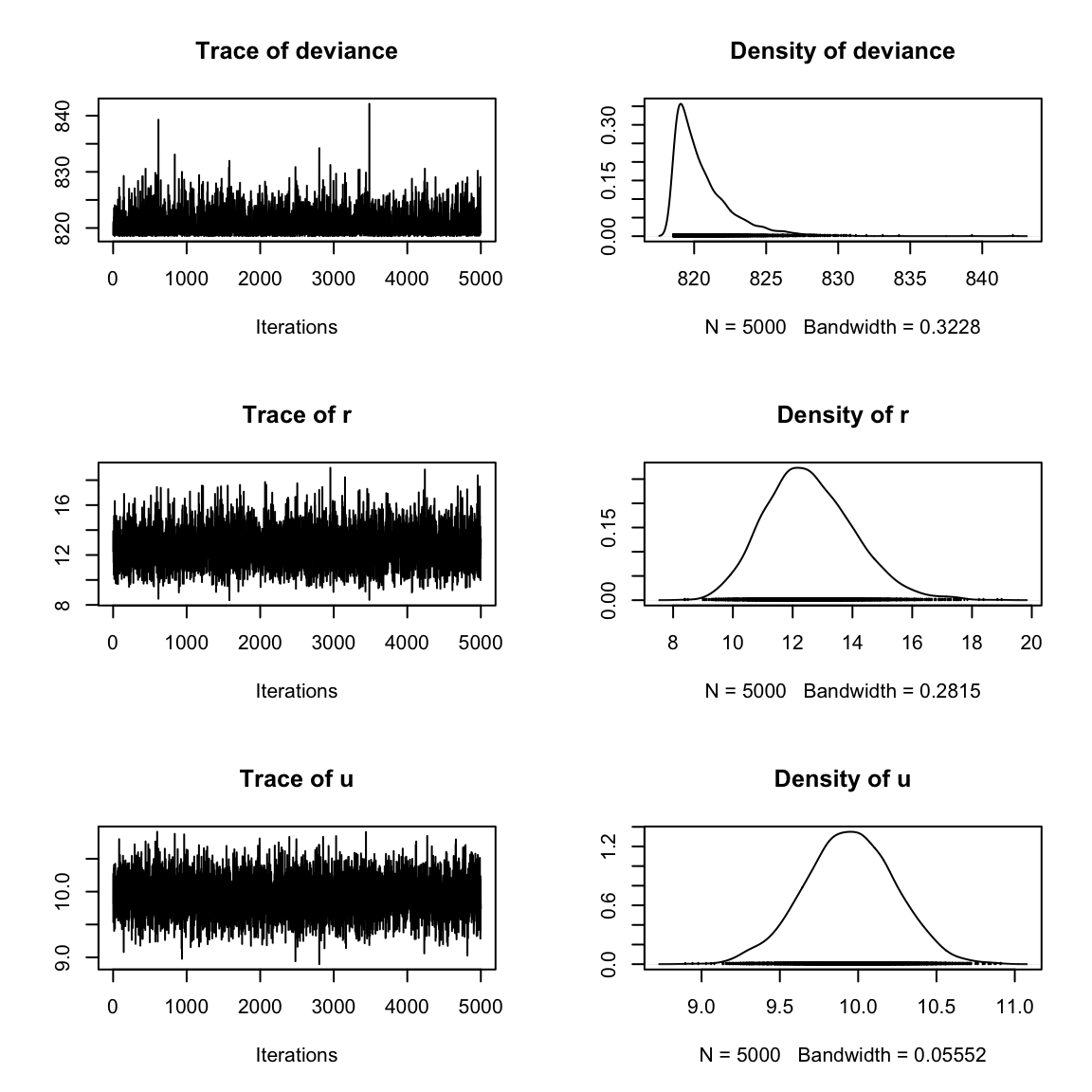
Figure 12.2: Plot of an object output from \(\texttt{creatMcmcList}\).
For more quantitative diagnostics of MCMC convergence, we can rely on the coda package in R. There are several useful statistics available, including the Gelman-Rubin diagnostic (for one or several chains), autocorrelation diagnostics (similar to the ACF you calculated above), the Geweke diagnostic, and Heidelberger-Welch test of stationarity.
library(coda)
gelmanDiags <- coda::gelman.diag(createMcmcList(mod_lm_intercept),
    multivariate = FALSE)
autocorDiags <- coda::autocorr.diag(createMcmcList(mod_lm_intercept))
gewekeDiags <- coda::geweke.diag(createMcmcList(mod_lm_intercept))
heidelDiags <- coda::heidel.diag(createMcmcList(mod_lm_intercept))
12.2.2 Linear regression with covariates
We can introduce Temp as the covariate explaining our response variable Wind. Our new equation is
\[\begin{equation} \begin{gathered} x_t = u + C\,c_t\\ y_t = x_t + v_t, v_t \sim \,\text{N}(0, r) \end{gathered} \tag{12.3} \end{equation}\]
To create JAGS code for this model, we (1) add a prior for our new parameter C, (2) update X[i] equation to include the new covariate, and (3) we include the new covariate in our named data list.
# 1. LINEAR REGRESSION with covariates

model.loc <- ("lm_covariate.txt")
jagsscript <- cat("
model {
   # priors on parameters
   u ~ dnorm(0, 0.01);
   C ~ dnorm(0,0.01);
   inv.r ~ dgamma(0.001,0.001);
   r <- 1/inv.r;

   # likelihood
   for(i in 1:N) {
      X[i] <- u + C*c[i];
      EY[i] <- X[i]
      Y[i] ~ dnorm(EY[i], inv.r);
   }
}
",
    file = model.loc)

jags.data <- list(Y = Wind, N = N, c = Temp)
jags.params <- c("r", "EY", "u", "C")
mod_lm <- R2jags::jags(jags.data, parameters.to.save = jags.params,
    model.file = model.loc, n.chains = 3, n.burnin = 5000, n.thin = 1,
    n.iter = 10000, DIC = TRUE)
We can show the the posterior fits (the model fits) to the data. Here is a simple function whose arguments are one of our fitted models and the raw data. The function is:
plotModelOutput <- function(jagsmodel, Y) {
    # attach the model
    EY <- jagsmodel$BUGSoutput$sims.list$EY
    x <- seq(1, length(Y))
    summaryPredictions <- cbind(apply(EY, 2, quantile, 0.025),
        apply(EY, 2, mean), apply(EY, 2, quantile, 0.975))
    plot(Y, col = "white", ylim = c(min(c(Y, summaryPredictions)),
        max(c(Y, summaryPredictions))), xlab = "", ylab = "95% CIs of predictions and data",
        main = paste("JAGS results:", jagsmodel$model.file))
    polygon(c(x, rev(x)), c(summaryPredictions[, 1], rev(summaryPredictions[,
        3])), col = "grey70", border = NA)
    lines(summaryPredictions[, 2])
    points(Y)
}
We can use the function to plot the predicted posterior mean with 95% CIs, as well as the raw data. Note that the shading is for the CIs on the expected value of \(y_t\) so will look narrow relative to the data. For example, try
plotModelOutput(mod_lm, Wind)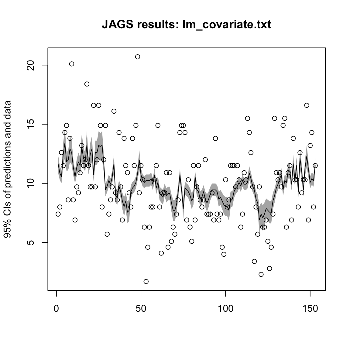
Figure 12.3: Predicted posterior mean with 95% CIs
12.2.3 Random walk with drift
The previous models were observation error only models. Switching gears, we can create process error models. We will start with a random walk model. In this model, the assumption is that the underlying state \(x_t\) is measured perfectly. All stochasticity is originating from process variation: variation in \(x_t\) to \(x_{t+1}\).
For this simple model, we will assume that wind behaves as a random walk. We will call this process \(x\) to prepare for the state-space model to come. We have no \(y_t\) part of the equation in this model.
\[\begin{equation} x_t = x_{t-1} + u + w_t, \text{ where }w_t \sim \,\text{N}(0,q) \tag{12.4} \end{equation}\] Now \(x_t\) is stochastic and \(E[X_t] = x_{t-1} + u\) and \(X_t \sim \,\text{N}(E[X_t],q)\).
We are going to need to put a prior on \(x_0\), which appears in \(E[X_1]\). We could start with \(t=2\) and skip this but we will start at \(t=1\) since we will need to do that for later problems. The question is what prior should we put on \(x_0\)? This is not a stationary process. We will just put a vague prior on \(x_0\).
The JAGS random walk model is:
# RANDOM WALK with drift

model.loc <- ("rw_intercept.txt")
jagsscript <- cat("
model {
   # priors on parameters
   u ~ dnorm(0, 0.01);
   inv.q ~ dgamma(0.001,0.001);
   q <- 1/inv.q;
   X0 ~ dnorm(0, 0.001);

   # likelihood
   X[1] ~ dnorm(X0 + u, inv.q);
   for(i in 2:N) {
      X[i] ~ dnorm(X[i-1] + u, inv.q);
   }
}
",
    file = model.loc)
To fit this model, we need to change jags.data to pass in X = Wind instead of Y = Wind. Obvioously we could have written the JAGS code with Y in place of X and kept our jags.data code the same as before, but we are working up to a state-space model where we have a hidden random walk called X and an observation of that called Y.
jags.data <- list(X = Wind, N = N)
jags.params <- c("q", "u")
mod_rw_intercept <- R2jags::jags(jags.data, parameters.to.save = jags.params,
    model.file = model.loc, n.chains = 3, n.burnin = 5000, n.thin = 1,
    n.iter = 10000, DIC = TRUE)
12.2.4 Autoregressive AR(1) time series models
A variation of the random walk model is the autoregressive time series model of order 1, AR(1). This model introduces a coefficient, which we will call \(b\). The parameter \(b\) controls the degree to which the random walk reverts to the mean. When \(b = 1\), the model is identical to the random walk, but at smaller values, the model will revert back to the mean (which in this case is zero). Also, \(b\) can take on negative values.
\[\begin{equation} x_t = b \, x_{t-1} + u + w_t, \text{ where }w_t \sim \,\text{N}(0,q) \tag{12.5} \end{equation}\] Now \(E[X_t] = b \, x_{t-1} + u\).
Once again we need to put a prior on \(x_0\), which appears in \(E[X_1]\). An AR(1) with \(|b|<1\) is a stationary process and the variance of the stationary distribution of \(x_t\) is \(q/(1-b^2)\). If you think that \(x_0\) has the stationary distribution (does your data look stationary?) then you can use the variance of the stationary distribution of \(x_t\) for your prior. We specify priors with the precision (1 over the variance) instead of the variance. Thus the precision of the stationary distribution of \(x_0\) is \((1/q)(1-b^2)\). In the code, inv.q is \(1/q\) and the precision is inv.q * (1-b*b).
# AR(1) MODEL WITH AND ESTIMATED AR COEFFICIENT

model.loc <- ("ar1_intercept.txt")
jagsscript <- cat("
model {
   # priors on parameters
   u ~ dnorm(0, 0.01);
   inv.q ~ dgamma(0.001,0.001);
   q <- 1/inv.q;
   b ~ dunif(-1,1);
   X0 ~ dnorm(0, inv.q * (1 - b * b));

   # likelihood
   X[1] ~ dnorm(b * X0 + u, inv.q);
   for(t in 2:N) {
      X[t] ~ dnorm(b * X[t-1] + u, inv.q);
   }
}
",
    file = model.loc)

jags.data <- list(X = Wind, N = N)
jags.params <- c("q", "u", "b")
mod_ar1_intercept <- R2jags::jags(jags.data, parameters.to.save = jags.params,
    model.file = model.loc, n.chains = 3, n.burnin = 5000, n.thin = 1,
    n.iter = 10000, DIC = TRUE)
12.2.5 Regression with AR(1) errors
The AR(1) model in the previous section suggests a way that we could include correlated errors in our linear regression. We could use the \(x_t\) AR(1) process as our errors for \(y_t\). Here is an example of modifying the intercept only linear regression model. We will set \(u\) to 0 so that our AR(1) errors have a mean of 0.
\[\begin{equation} \begin{gathered} x_t = b \, x_{t-1} + w_t, \text{ where }w_t \sim \,\text{N}(0,q) \\ y_t = a + x_t \end{gathered} \tag{12.6} \end{equation}\]
The problem with this is that we need a distribution for \(y_t\). We cannot use Y[t] <- a + X[t] in our JAGS code (\(Y_t\) is a random varible with a distribution; you cannot assign it a value). We need to re-write this as \(Y_t \sim N(a + b \, x_{t-1}, q)\).
\[\begin{equation} \begin{gathered} Y_t \sim N(a + b \, x_{t-1}, q) \\ x_t = y_t - a \end{gathered} \tag{12.7} \end{equation}\]
We will create the variable EY so we can keep track of the expected value of \(Y_t\), conditioned on \(t-1\).
# LINEAR REGRESSION with autocorrelated errors no
# covariates, intercept only.

model.loc <- ("lm_intercept_ar1b.txt")
jagsscript <- cat("
model {
   # priors on parameters
   a ~ dnorm(0, 0.01);
   inv.q ~ dgamma(0.001,0.001);
   q <- 1/inv.q;
   b ~ dunif(-1,1);
   X0 ~ dnorm(0, inv.q * (1 - b * b));

   # likelihood
   EY[1] <- a + b * X0;
   Y[1] ~ dnorm(EY[1], inv.q);
   X[1] <- Y[1] - a;
   for(t in 2:N) {
      EY[t] <- a + b * X[t-1];
      Y[t] ~ dnorm(EY[1], inv.q);
      X[t] <- Y[t]-a;
   }
}
",
    file = model.loc)

jags.data <- list(Y = Wind, N = N)
jags.params <- c("q", "EY", "a", "b")
mod_ar1_intercept <- R2jags::jags(jags.data, parameters.to.save = jags.params,
    model.file = model.loc, n.chains = 3, n.burnin = 5000, n.thin = 1,
    n.iter = 10000, DIC = TRUE)
12.2.6 Univariate state space model
Now we will combine the process and observation models to create a univariate state-space model. This is the classic stochastic level model.
\[\begin{equation} \begin{gathered} x_t = x_{t-1} + u + w_t, \, w_t \sim N(0,q)\\ y_t = x_t + v_t, \, v_t \sim \,\text{N}(0, r) \end{gathered} \tag{12.8} \end{equation}\]
Because \(x\) is a random walk model not a stationary AR(1), we will place a vague weakly informative prior on \(x_0\): \(x_0 \sim \,\text{N}(y_1, 1000)\). We had to pass in Y1 as data because JAGS would complain if we used Y[1] in our prior (because have X0 in our model for \(Y[1]\)). EY is added so that we can track the model fits for \(y\). In this case it is just X but in more complex models it will involve more parameters.
model.loc <- ("ss_model.txt")
jagsscript <- cat("
model {
   # priors on parameters
   u ~ dnorm(0, 0.01);
   inv.q ~ dgamma(0.001,0.001);
   q <- 1/inv.q;
   inv.r ~ dgamma(0.001,0.001);
   r <- 1/inv.r;
   X0 ~ dnorm(Y1, 0.001);

   # likelihood
   X[1] ~ dnorm(X0 + u, inv.q);
   EY[1] <- X[1];
   Y[1] ~ dnorm(EY[1], inv.r);
   for(t in 2:N) {
      X[t] ~ dnorm(X[t-1] + u, inv.q);
      EY[t] <- X[t];
      Y[t] ~ dnorm(EY[t], inv.r);
   }
}
",
    file = model.loc)
We fit as usual with the addition of Y1 in jags.data.
jags.data <- list(Y = Wind, N = N, Y1 = Wind[1])
jags.params <- c("q", "r", "EY", "u")
mod_ss <- jags(jags.data, parameters.to.save = jags.params, model.file = model.loc,
    n.chains = 3, n.burnin = 5000, n.thin = 1, n.iter = 10000,
    DIC = TRUE)