16.3 Modeling the cycle

As discussed in Chapter 15 in the covariates chapter, we can model changes in seasonality with a DLM with sine and cosine covariates. Here is a DLM model with the level and season modeled as a random walk.

\[\begin{bmatrix}x \\ \beta_1 \\ \beta_2 \end{bmatrix}_t = \begin{bmatrix}x \\ \beta_1 \\ \beta_2 \end{bmatrix}_{t-1} + \begin{bmatrix}w_1 \\ w_2 \\ w_3 \end{bmatrix}_t\] \[y_t = \begin{bmatrix}1& \sin(2\pi t/p)&\cos(2\pi t/p)\end{bmatrix} \begin{bmatrix}x \\ \beta_1 \\ \beta_2 \end{bmatrix}_t + v_t\]

We can fit the model to the Kvichak River log spawner data and estimate the \(\beta\)’s and stochastic level (\(x\)). This is annual data so what does \(p\) mean? \(p\) is the time steps between peaks. For sockeye that is 5 years. So we set \(p=5\). If \(p\) were changing, that would cause problems, but it is not for these data (which you can confirm by looking at the ACF for different parts of the time series).

16.3.1 Set up the data

river <- "KVICHAK"
df <- subset(sockeye, region == river)
yt <- log(df$spawners)
TT <- length(yt)
p <- 5

16.3.2 Specify the \(\mathbf{Z}\) matrix

\(\mathbf{Z}\) is time-varying and we set this up with an array with the 3rd dimension being time.

Z <- array(1, dim = c(1, 3, TT))
Z[1, 2, ] <- sin(2 * pi * (1:TT)/p)
Z[1, 3, ] <- cos(2 * pi * (1:TT)/p)

16.3.3 Specify the model list

Then we make our model list. We need to set \(\mathbf{A}\) since MARSS() doesn’t like the default value of scaling when \(\mathbf{Z}\) is time-varying.

mod.list <- list(U = "zero", Q = "diagonal and unequal", Z = Z, 
    A = "zero")

16.3.4 Fit the model

When we fit the model we need to give MARSS() initial values for x0. It cannot come up with default ones for this model. It doesn’t really matter what you pick.

m <- dim(Z)[2]
fit <- MARSS(yt, model = mod.list, inits = list(x0 = matrix(0, 
    m, 1)))

Warning! Abstol convergence only. Maxit (=500) reached before log-log convergence.

MARSS fit is
Estimation method: kem 
Convergence test: conv.test.slope.tol = 0.5, abstol = 0.001
WARNING: Abstol convergence only no log-log convergence.
 maxit (=500) reached before log-log convergence.
 The likelihood and params might not be at the ML values.
 Try setting control$maxit higher.
Log-likelihood: -58.61614 
AIC: 131.2323   AICc: 133.899   
 
           Estimate
R.R        0.415426
Q.(X1,X1)  0.012584
Q.(X2,X2)  0.000547
Q.(X3,X3)  0.037008
x0.X1      7.897380
x0.X2     -0.855359
x0.X3      1.300854
Initial states (x0) defined at t=0

Standard errors have not been calculated. 
Use MARSSparamCIs to compute CIs and bias estimates.

Convergence warnings
 Warning: the  Q.(X2,X2)  parameter value has not converged.
 Type MARSSinfo("convergence") for more info on this warning.

16.3.5 Plot the output

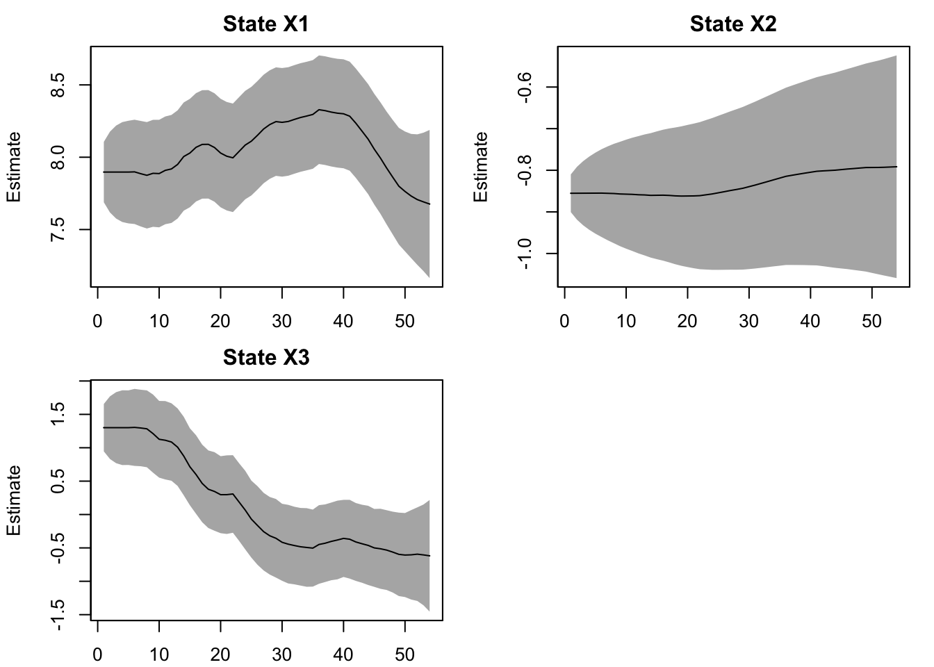
The \(\beta_1\) estimate is State X2 and \(\beta_2\) is State X3. The estimates match what we put into the simulated data.

plot type = "xtT" Estimated states

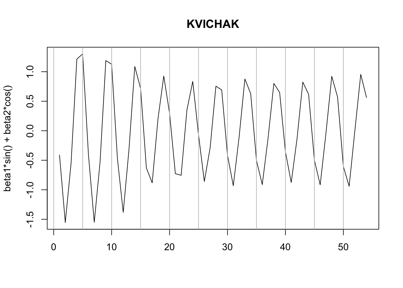
We can plot our cycle estimates and see that the peak has shifted over time. The peak has not been regularly every 5 years.

Let’s look at the other rivers. Write a function to do the fit.

fitriver <- function(river, p = 5) {
    df <- subset(sockeye, region == river)
    yt <- log(df$spawners)
    TT <- length(yt)
    Z <- array(1, dim = c(1, 3, TT))
    Z[1, 2, ] <- sin(2 * pi * (1:TT)/p)
    Z[1, 3, ] <- cos(2 * pi * (1:TT)/p)
    mod.list <- list(U = "zero", Q = "diagonal and unequal", 
        Z = Z, A = "zero")
    fit <- MARSS(yt, model = mod.list, inits = list(x0 = matrix(0, 
        3, 1)), silent = TRUE)
    return(fit)
}

The make a list with all the fits.

fits <- list()
for (river in names(a)) {
    fits[[river]] <- fitriver(river)
}

Create a data frame of the amplitude of the cycle (\(\sqrt{\beta_1^2+\beta_2^2}\)) and the stochastic level (\(x\)).

dfz <- data.frame()
for (river in names(a)) {
    fit <- fits[[river]]
    tmp <- data.frame(amplitude = sqrt(fit$states[2, ]^2 + fit$states[3, 
        ]^2), trend = fit$states[1, ], river = river, brood_year = subset(sockeye, 
        region == river)$brood_year)
    dfz <- rbind(dfz, tmp)
}