7.2 West coast harbor seals counts

In this example, we will use multivariate state-space models to combine surveys from four survey regions to estimate the average long-term population growth rate and the year-to-year variability in that population growth rate.

We have five regions (or sites) where harbor seals were censused from 1978-1999 while hauled out of land. During the period of this dataset, harbor seals were recovering steadily after having been reduced to low levels by hunting prior to protection. We will assume that the underlying population process is a stochastic exponential growth process with mean rates of increase that were not changing through 1978-1999.

The survey methodologies were consistent throughout the 20 years of the data but we do not know what fraction of the population that each region represents nor do we know the observation-error variance for each region. Given differences between the numbers of haul-outs in each region, the observation errors may be quite different. The regions have had different levels of sampling; the best sampled region has only 4 years missing while the worst has over half the years missing (Figure 7.1).

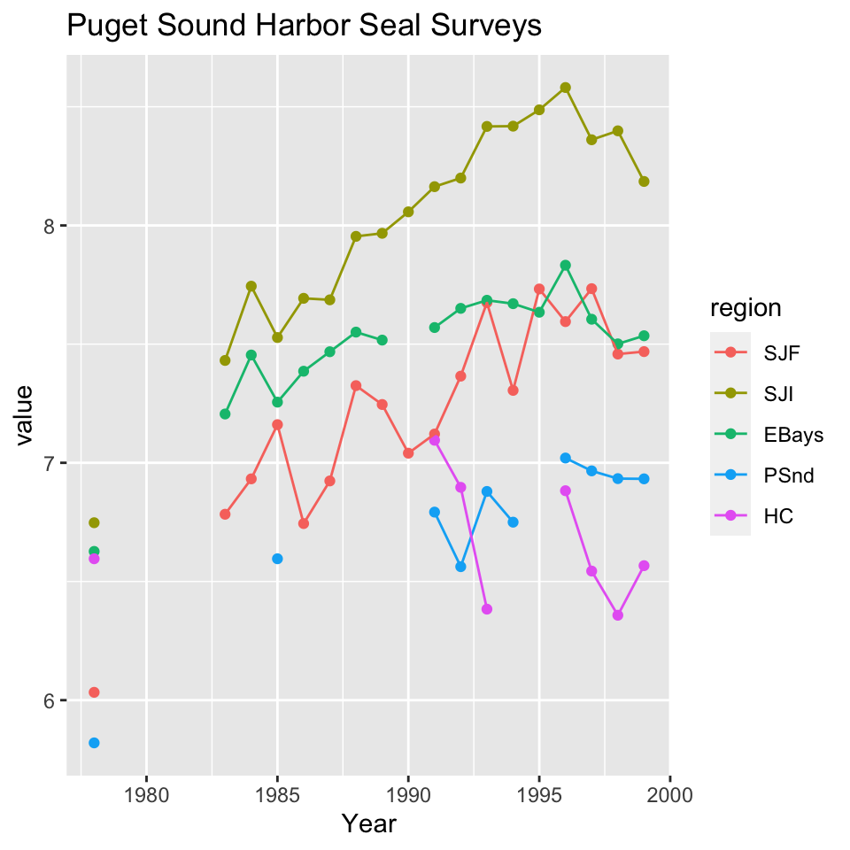
Plot of the of the count data from the five harbor seal regions (Jeffries et al. 2003). The numbers on each line denote the different regions: 1) Strait of Juan de Fuca (SJF), 2) San Juan Islands (SJI), 2) Eastern Bays (EBays), 4) Puget Sound (PSnd), and 5) Hood Canal (HC). Each region is an index of the total harbor seal population in each region.

Figure 7.1: Plot of the of the count data from the five harbor seal regions (Jeffries et al. 2003). The numbers on each line denote the different regions: 1) Strait of Juan de Fuca (SJF), 2) San Juan Islands (SJI), 2) Eastern Bays (EBays), 4) Puget Sound (PSnd), and 5) Hood Canal (HC). Each region is an index of the total harbor seal population in each region.

7.2.1 Load the harbor seal data

The harbor seal data are included in the MARSS package as matrix with years in column 1 and the logged counts in the other columns. Let’s look at the first few years of data:

data(harborSealWA, package = "MARSS")
print(harborSealWA[1:8, ], digits = 3)

     Year  SJF  SJI EBays PSnd  HC
[1,] 1978 6.03 6.75  6.63 5.82 6.6
[2,] 1979   NA   NA    NA   NA  NA
[3,] 1980   NA   NA    NA   NA  NA
[4,] 1981   NA   NA    NA   NA  NA
[5,] 1982   NA   NA    NA   NA  NA
[6,] 1983 6.78 7.43  7.21   NA  NA
[7,] 1984 6.93 7.74  7.45   NA  NA
[8,] 1985 7.16 7.53  7.26 6.60  NA

We are going to leave out Hood Canal (HC) since that region is somewhat isolated from the others and experiencing very different conditions due to hypoxic events and periodic intense killer whale predation. We will set up the data as follows:

dat <- MARSS::harborSealWA
years <- dat[, "Year"]
dat <- dat[, !(colnames(dat) %in% c("Year", "HC"))]
dat <- t(dat)  # transpose to have years across columns
colnames(dat) <- years
n <- nrow(dat) - 1