4.8 Moving-average (MA) models

A moving-averge process of order \(q\), or MA(\(q\)), is a weighted sum of the current random error plus the \(q\) most recent errors, and can be written as

\[\begin{equation} \tag{4.22} x_t = w_t + \theta_1 w_{t-1} + \theta_2 w_{t-2} + \dots + \theta_q w_{t-q}, \end{equation}\]

where \(\{w_t\}\) is a white noise sequence with zero mean and some variance \(\sigma^2\); for our purposes we usually assume that \(w_t \sim \text{N}(0,q)\). Of particular note is that because MA processes are finite sums of stationary errors, they themselves are stationary.

Of interest to us are so-called “invertible” MA processes that can be expressed as an infinite AR process with no error term. The term invertible comes from the inversion of the backshift operator (B) that we discussed in class (i.e., \(\mathbf{B} x_t= x_{t-1}\)). So, for example, an MA(1) process with \(\theta < \lvert 1 \rvert\) is invertible because it can be written using the backshift operator as

\[\begin{equation} \tag{4.23} \begin{aligned} x_t &= w_t - \theta w_{t-1} \\ x_t &= w_t - \theta \mathbf{B} w_t \\ x_t &= (1 - \theta \mathbf{B}) w_t, \\ &\Downarrow \\ w_t &= \frac{1}{(1 - \theta \mathbf{B})} x_t \\ w_t &= (1 + \theta \mathbf{B} + \theta^2 \mathbf{B}^2 + \theta^3 \mathbf{B}^3 + \dots) x_t \\ w_t &= x_t + \theta x_{t-1} + \theta^2 x_{t-2} + \theta^3 x_{t-3} + \dots \end{aligned} \end{equation}\]

4.8.1 Simulating an MA(\(q\)) process

We can simulate MA(\(q\)) processes just as we did for AR(\(p\)) processes using arima.sim(). Here are 3 different ones with contrasting \(\theta\)’s:

set.seed(123)
## list description for MA(1) model with small coef
MA_sm <- list(order = c(0, 0, 1), ma = 0.2)
## list description for MA(1) model with large coef
MA_lg <- list(order = c(0, 0, 1), ma = 0.8)
## list description for MA(1) model with large coef
MA_neg <- list(order = c(0, 0, 1), ma = -0.5)
## simulate MA(1)
MA1_sm <- arima.sim(n = 50, model = MA_sm, sd = 0.1)
MA1_lg <- arima.sim(n = 50, model = MA_lg, sd = 0.1)
MA1_neg <- arima.sim(n = 50, model = MA_neg, sd = 0.1)

with their associated plots.

## setup plot region
par(mfrow = c(1, 3))
## plot the ts
plot.ts(MA1_sm, ylab = expression(italic(x)[italic(t)]), main = expression(paste(theta, 
    " = 0.2")))
plot.ts(MA1_lg, ylab = expression(italic(x)[italic(t)]), main = expression(paste(theta, 
    " = 0.8")))
plot.ts(MA1_neg, ylab = expression(italic(x)[italic(t)]), main = expression(paste(theta, 
    " = -0.5")))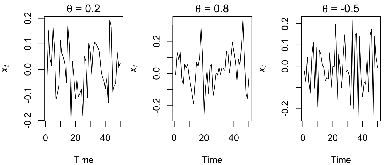

Figure 4.25: Time series of simulated MA(1) processes with \(\theta=0.2\) (left), \(\theta=0.8\) (middle), and \(\theta=-0.5\) (right).

In contrast to AR(1) processes, MA(1) models do not exhibit radically different behavior with changing \(\theta\). This should not be too surprising given that they are simply linear combinations of white noise.

4.8.2 Correlation structure of MA(\(q\)) processes

We saw in lecture and above how the ACF and PACF have distinctive features for AR(\(p\)) models, and they do for MA(\(q\)) models as well. Here are examples of four MA(\(q\)) processes. As before, we’ll use a really big \(n\) so as to make them “pure,” which will provide a much better estimate of the correlation structure.

set.seed(123)
## the 4 MA coefficients
MA_q_coef <- c(0.7, 0.2, -0.1, -0.3)
## empty list for storing models
MA_mods <- list()
## loop over orders of q
for (q in 1:4) {
    ## assume sd = 1, so not specified
    MA_mods[[q]] <- arima.sim(n = 1000, list(ma = MA_q_coef[1:q]))
}

Now that we have our four MA(\(q\)) models, lets look at plots of the time series, ACF’s, and PACF’s.

## set up plot region
par(mfrow = c(4, 3))
## loop over orders of q
for (q in 1:4) {
    plot.ts(MA_mods[[q]][1:50], ylab = paste("MA(", q, ")", sep = ""))
    acf(MA_mods[[q]], lag.max = 12)
    pacf(MA_mods[[q]], lag.max = 12, ylab = "PACF")
}

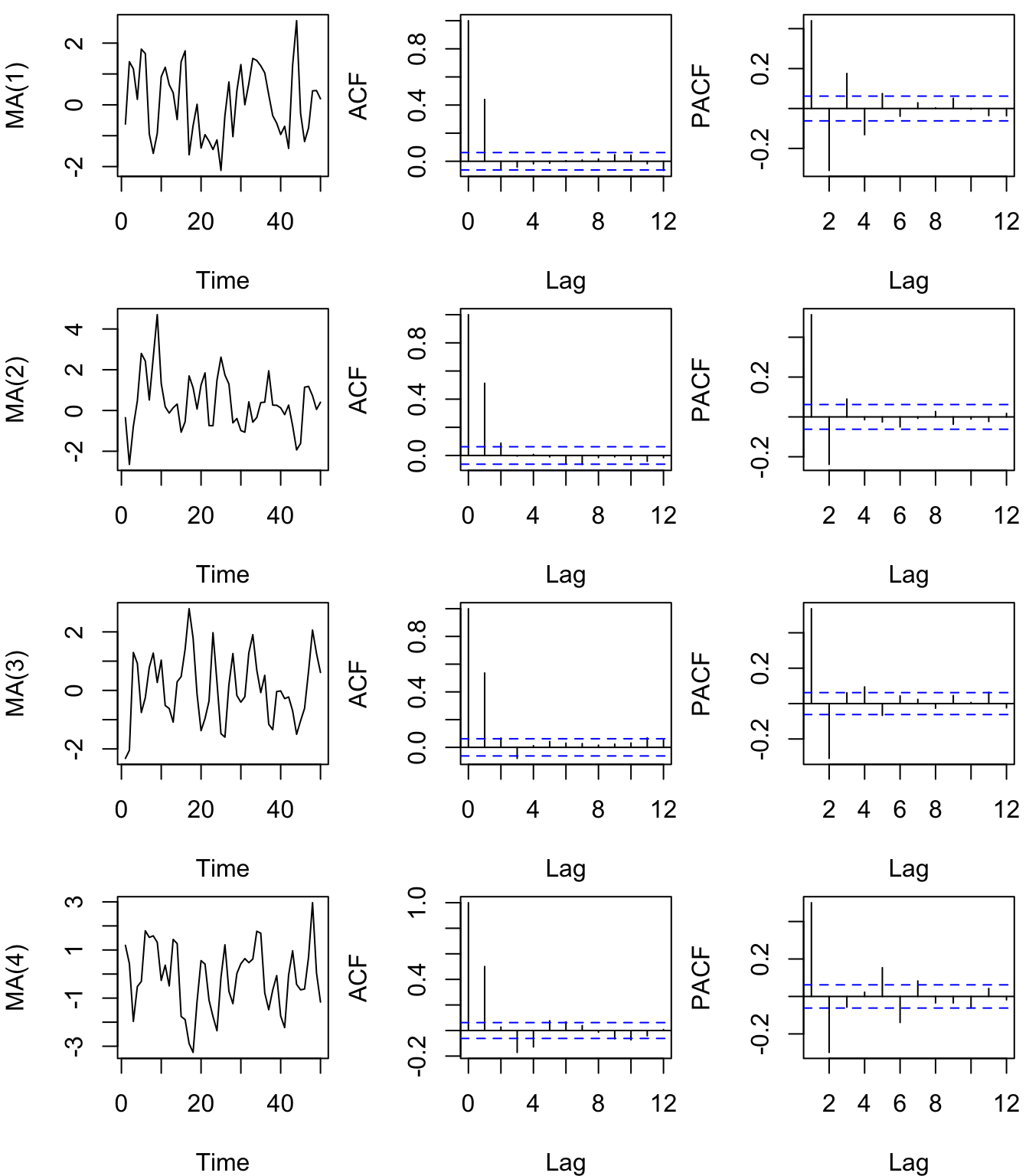
Figure 4.26: Time series of simulated MA(\(q\)) processes (left column) of increasing orders from 1-4 (rows) with their associated ACF’s (center column) and PACF’s (right column). Note that only the first 50 values of \(x_t\) are plotted.

Note very little qualitative difference in the realizations of the four MA(\(q\)) processes (Figure 4.26). As we saw in lecture and is evident from our examples here, however, the ACF for an MA(\(q\)) process goes to zero for lags > \(q\), but the PACF tails off toward zero very slowly. This is an important diagnostic tool when trying to identify the order of \(q\) in ARMA(\(p,q\)) models.