6.2 Examples using the Nile river data
We will use the data from the Nile River (Figure 6.1). We will fit different flow models to the data and compare the models with AIC.
library(datasets)
dat <- Nile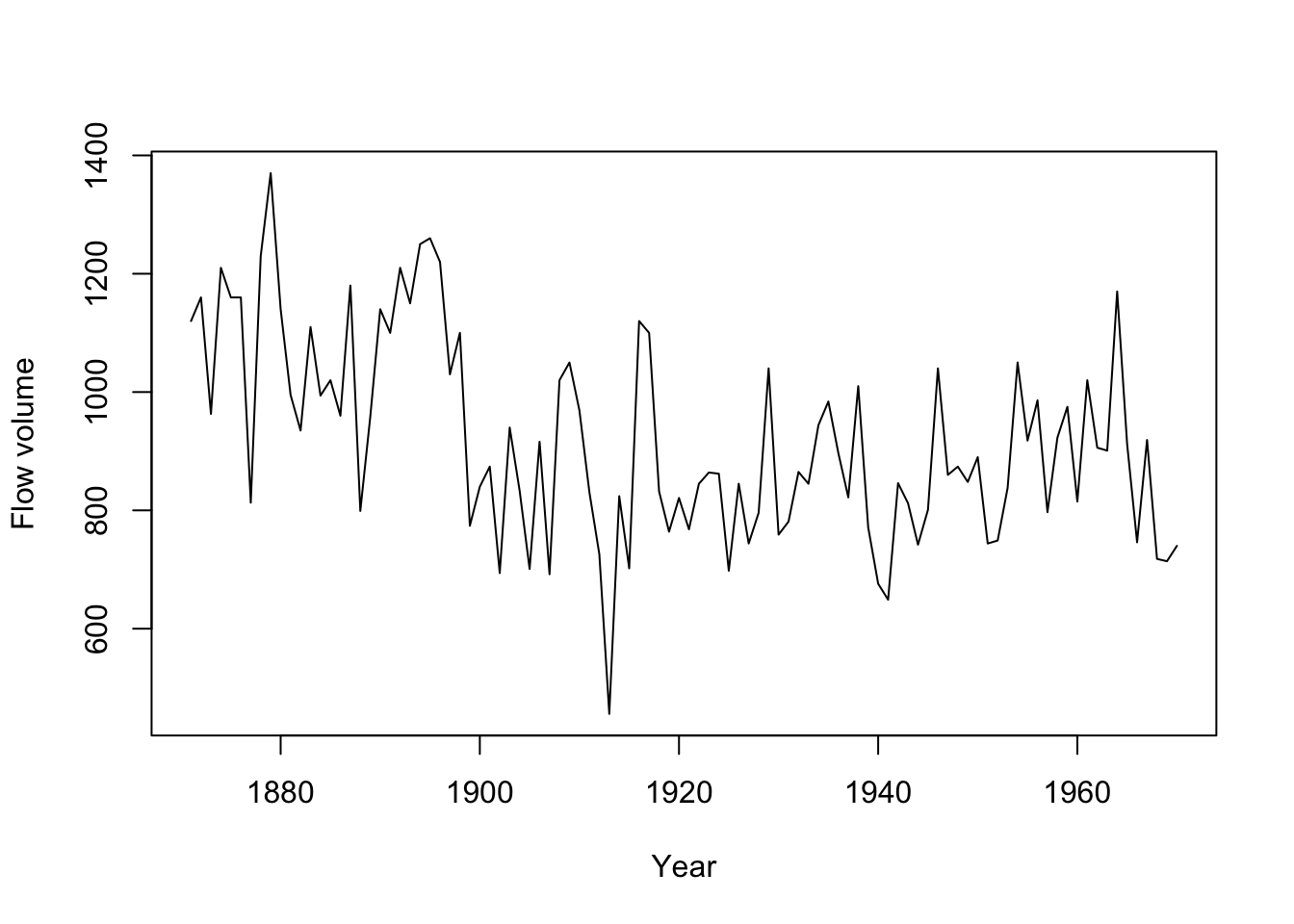
Figure 6.1: The Nile River flow volume 1871 to 1970 (Nile dataset in R).
6.2.1 Flat level model
We will start by modeling these data as a simple average river flow with variability around some level \(\mu\).
\[\begin{equation}
y_t = \mu + v_t \text{ where } v_t \sim \,\text{N}(0,r)
\tag{6.3}
\end{equation}\]
where \(y_t\) is the river flow volume at year \(t\).
We can write this model as a univariate state-space model as follows. We use \(x_t\) to model the average flow level. \(y_t\) is just an observation of this flat \(x_t\). Work through \(x_1\), \(x_2\), \(\dots\) starting from \(x_0\) to convince yourself that \(x_t\) will always equal \(\mu\). \[\begin{equation} \begin{gathered} x_t = 1 \times x_{t-1}+ 0 + w_t \text{ where } w_t \sim \,\text{N}(0,0) \\ y_t = 1 \times x_t + 0 + v_t \text{ where } v_t \sim \,\text{N}(0,r) \\ x_0 = \mu \end{gathered} \tag{6.4} \end{equation}\] The model is specified as a list as follows:
mod.nile.0 <- list(B = matrix(1), U = matrix(0), Q = matrix(0),
    Z = matrix(1), A = matrix(0), R = matrix("r"), x0 = matrix("mu"),
    tinitx = 0)
We then fit the model:
kem.0 <- MARSS(dat, model = mod.nile.0)Output not shown, but here are the estimates and AICc.
c(coef(kem.0, type = "vector"), LL = kem.0$logLik, AICc = kem.0$AICc) R.r x0.mu LL AICc
28351.5675 919.3500 -654.5157 1313.1552 6.2.2 Linear trend in flow model
Figure 6.2 shows the fit for the flat average river flow model. Looking at the data, we might expect that a declining average river flow would be better. In MARSS form, that model would be: \[\begin{equation} \begin{gathered} x_t = 1 \times x_{t-1}+ u + w_t \text{ where } w_t \sim \,\text{N}(0,0) \\ y_t = 1 \times x_t + 0 + v_t \text{ where } v_t \sim \,\text{N}(0,r) \\ x_0 = \mu \end{gathered} \tag{6.5} \end{equation}\] where \(u\) is now the average per-year decline in river flow volume. The model is specified as follows:
mod.nile.1 <- list(B = matrix(1), U = matrix("u"), Q = matrix(0),
    Z = matrix(1), A = matrix(0), R = matrix("r"), x0 = matrix("mu"),
    tinitx = 0)
We then fit the model:
kem.1 <- MARSS(dat, model = mod.nile.1)Here are the estimates, log-likelihood and AICc:
c(coef(kem.1, type = "vector"), LL = kem.1$logLik, AICc = kem.1$AICc) R.r U.u x0.mu LL AICc
22213.595453 -2.692106 1054.935067 -642.315910 1290.881821 Figure 6.2 shows the fits for the two models with deterministic models (flat and declining) for mean river flow along with their AICc values (smaller AICc is better). The AICc for the model with a declining river flow is lower by over 20 (which is a lot).
6.2.3 Stochastic level model
Looking at the flow levels, we might suspect that a model that allows the average flow to change would model the data better and we might suspect that there have been sudden, and anomalous, changes in the river flow level.
We will now model the average river flow at year \(t\) as a random walk, specifically an autoregressive process which means that average river flow is year \(t\) is a function of average river flow in year \(t-1\).
\[\begin{equation}
\begin{gathered}
x_t = x_{t-1}+w_t \text{ where } w_t \sim \,\text{N}(0,q) \\
y_t = x_t+v_t \text{ where } v_t \sim \,\text{N}(0,r) \\
x_0 = \mu
\end{gathered}
\tag{6.6}
\end{equation}\]
As before, \(y_t\) is the river flow volume at year \(t\). \(x_t\) is the mean level.
The model is specified as:
mod.nile.2 <- list(B = matrix(1), U = matrix(0), Q = matrix("q"),
    Z = matrix(1), A = matrix(0), R = matrix("r"), x0 = matrix("mu"),
    tinitx = 0)
We could also use the text shortcuts to specify the model. Because \(\mathbf{R}\) and \(\mathbf{Q}\) are \(1 \times 1\) matrices, “unconstrained,” “diagonal and unequal,” “diagonal and equal” and “equalvarcov” will all lead to a \(1 \times 1\) matrix with one estimated element. For \(\mathbf{a}\) and \(\mathbf{u}\), the following shortcut could be used:
A <- "zero"
U <- "zero"
Because \(\mathbf{x}_0\) is \(1 \times 1\), it could be specified as “unequal,” “equal” or “unconstrained.”
kem.2 <- MARSS(dat, model = mod.nile.2)Here are the estimates, log-likelihood and AICc:
c(coef(kem.2, type = "vector"), LL = kem.2$logLik, AICc = kem.2$AICc) R.r Q.q x0.mu LL AICc
15065.6121 1425.0030 1111.6338 -637.7631 1281.7762 6.2.4 Stochastic level model with drift
We can add a drift to term to our random walk; the \(u\) in the process model (\(x\)) is the drift term. This causes the random walk to tend to trend up or down.
\[\begin{equation}
\begin{gathered}
x_t = x_{t-1}+u+w_t \text{ where } w_t \sim \,\text{N}(0,q) \\
y_t = x_t+v_t \text{ where } v_t \sim \,\text{N}(0,r) \\
x_0 = \mu
\end{gathered}
\tag{6.7}
\end{equation}\]
The model is then specified by changing U to indicate that a \(u\) is estimated:
mod.nile.3 <- list(B = matrix(1), U = matrix("u"), Q = matrix("q"),
    Z = matrix(1), A = matrix(0), R = matrix("r"), x0 = matrix("mu"),
tinitx = 0)kem.3 <- MARSS(dat, model = mod.nile.3)Here are the estimates, log-likelihood and AICc:
c(coef(kem.3, type = "vector"), LL = kem.3$logLik, AICc = kem.3$AICc) R.r U.u Q.q x0.mu LL AICc
15585.278194 -3.248793 1088.987455 1124.044484 -637.302692 1283.026436 Figure 6.2 shows all the models along with their AICc values.