15.4 Time-varying amplitude

Instead of a constant seasonality, we can imagine that it varies in time. The first way it might vary is in the amplitude of the seasonality. So the location of the peak is the same but the difference between the peak and valley changes.

\[z_t\left(\beta_1 \sin(2 \pi t/p) + \beta_2 \cos(2 \pi t/p)\right)\]

In this case, the \(\beta\)’s remain constant but the sum of the sines and cosines is multiplied by a time-varying scaling factor.

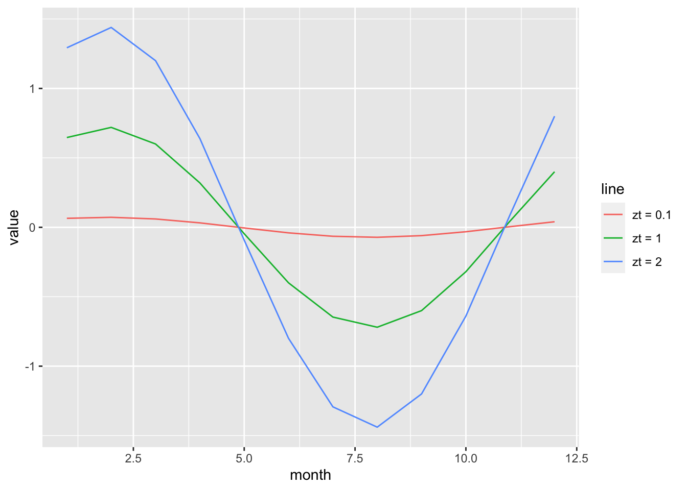
Here we simulate some data where \(z_t\) is sinusoidal and is largest in the beginning of the time-series. Note we want \(z_t\) to stay positive otherwise our peak will become a valley when \(z_t\) goes negative.

set.seed(1234)
TT <- 100
q <- 0.1
r <- 0.1
beta1 <- 0.6
beta2 <- 0.4
zt <- 0.5 * sin(2 * pi * (1:TT)/TT) + 0.75
cov1 <- sin(2 * pi * (1:TT)/12)
cov2 <- cos(2 * pi * (1:TT)/12)
xt <- cumsum(rnorm(TT, 0, q))
yt <- xt + zt * beta1 * cov1 + zt * beta2 * cov2 + rnorm(TT, 
    0, r)
plot(yt, type = "l", xlab = "t")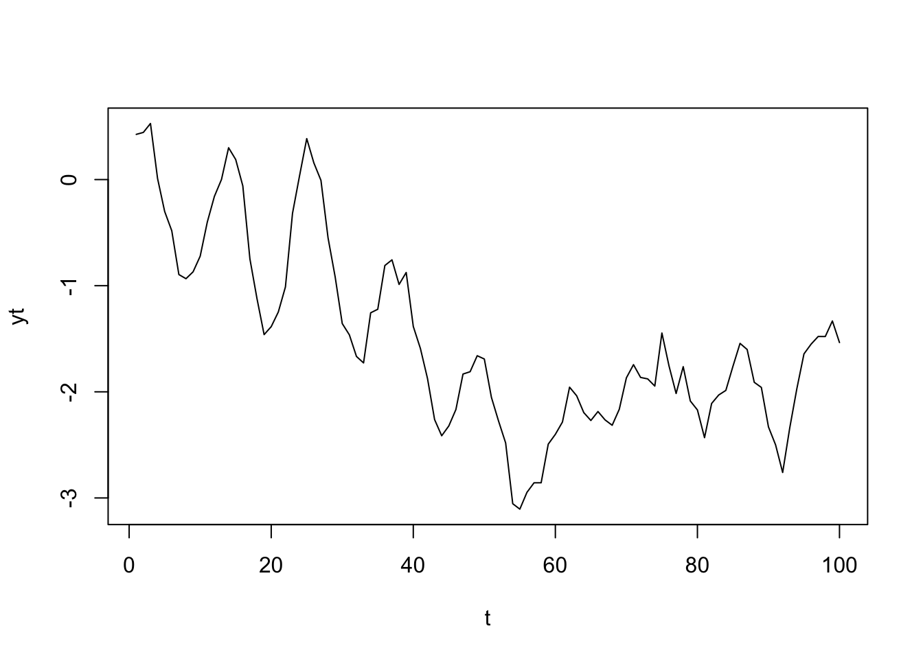

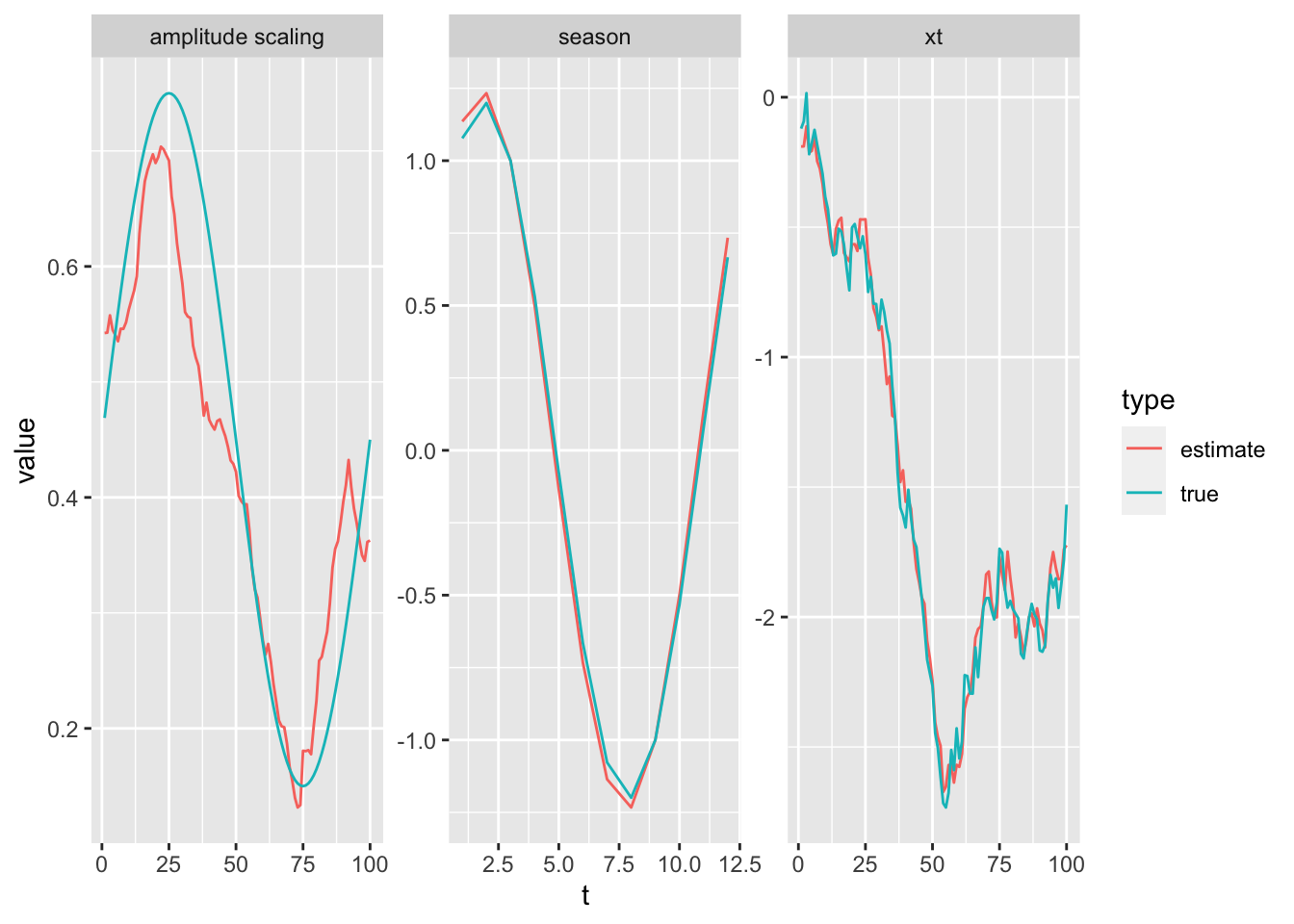
15.4.1 Fitting the model

When the seasonality is written as \[z_t\left(\beta_1 \sin(2 \pi t/p) + \beta_2 \cos(2 \pi t/p)\right)\] our model is under-determined because we have \(z_t \beta_1\) and \(z_t \beta_2\). We can scale the $z_t up and the \(\beta\)’s correspondingly down and have the same values (so multiply \(z_t\) by 2 and divide the \(\beta\)’s by 2, say). We can fix that by multiplying the \(z_t\) and dividing the seaonal part by \(\beta_1\). Then our seasonal model becomes Recognizing when your model is under-determined takes some experience. If you work in a Bayesian framework, it is a bit easier because it is easy to look at the posterior distributions and look for ridges.

\[(z_t/\beta_1) \left(\sin(2 \pi t/p) + (\beta_2/\beta_1) \cos(2 \pi t/p)\right) = \\ x_{2,t} \left(\sin(2 \pi t/p) + \beta \cos(2 \pi t/p)\right) \] The seasonality (peak location) will be the same for \((\sin(2 \pi t/p) + \beta \cos(2 \pi t/p))\) and \((\beta_1 \sin(2 \pi t/p) + \beta_2 \cos(2 \pi t/p))\). The only thing that is different is the amplitude and we are using \(x_{2,t}\) to determine the amplitude.

Now our \(x\) and \(y\) models look like this. Notice that the \(\mathbf{Z}\) is \(1 \times 2\) instead of \(1 \times 3\).

\[\begin{bmatrix}x_1 \\ x_2 \end{bmatrix}_t = \begin{bmatrix}x_1 \\ x_2 \end{bmatrix}_{t-1} + \begin{bmatrix}w_1 \\ w_2 \end{bmatrix}_t\]

\[y_t = \begin{bmatrix}1& \sin(2\pi t/p) + \beta \cos(2\pi t/p)\end{bmatrix} \begin{bmatrix}x_1 \\ x_2 \end{bmatrix}_t + v_t\]

To set up the Z matrix, we can pass in values like "1 + 0.5*beta". MARSS() will translate that to \(1+0.5\beta\).

Z <- array(list(1), dim = c(1, 2, TT))
Z[1, 2, ] <- paste0(sin(2 * pi * (1:TT)/12), " + ", cos(2 * pi * 
    (1:TT)/12), "*beta")

Then we make our model list. We need to set A since MARSS() doesn’t like the default value of scaling when Z is time-varying.

mod.list <- list(U = "zero", Q = "diagonal and unequal", Z = Z, 
    A = "zero")

require(MARSS)
fit <- MARSS(yt, model = mod.list, inits = list(x0 = matrix(0, 
    2, 1)))

We are able to recover the level, seasonality and changing amplitude of the seasonality.