9.9 Forecast diagnostics

In the literature on state-space models, the set of \(e_t\) are commonly referred to as “innovations.” MARSS() calculates the innovations as part of the Kalman filter algorithm—they are stored as Innov in the list produced by the MARSSkfss() function.

## forecast errors
innov <- kf_out$Innov

Let’s see if our innovations meet the model assumptions. Beginning with (1), we can use a Q-Q plot to see whether the innovations are normally distributed with a mean of zero. We’ll use the qqnorm() function to plot the quantiles of the innovations on the \(y\)-axis versus the theoretical quantiles from a Normal distribution on the \(x\)-axis. If the 2 distributions are similar, the points should fall on the line defined by \(y = x\).

## Q-Q plot of innovations
qqnorm(t(innov), main = "", pch = 16, col = "blue")
## add y=x line for easier interpretation
qqline(t(innov))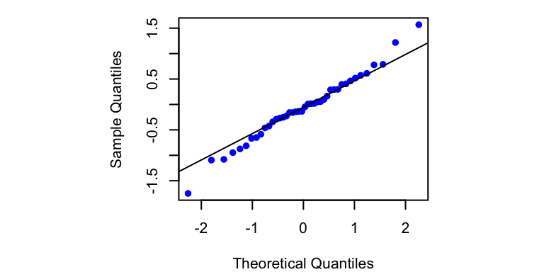

Figure 9.5: Q-Q plot of the forecast errors (innovations) for the DLM specified in Equations (9.19)–(9.21).

The Q-Q plot (Figure 9.5) indicates that the innovations appear to be more-or-less normally distributed (i.e., most points fall on the line). Furthermore, it looks like the mean of the innovations is about 0, but we should use a more reliable test than simple visual inspection. We can formally test whether the mean of the innovations is significantly different from 0 by using a one-sample \(t\)-test. based on a null hypothesis of \(\,\text{E}(e_t)=0\). To do so, we will use the function t.test() and base our inference on a significance value of \(\alpha = 0.05\).

## p-value for t-test of H0: E(innov) = 0
t.test(t(innov), mu = 0)$p.value

[1] 0.4840901

The \(p\)-value \(>>\) 0.05 so we cannot reject the null hypothesis that \(\,\text{E}(e_t)=0\).

Moving on to assumption (2), we can use the sample autocorrelation function (ACF) to examine whether the innovations covary with a time-lagged version of themselves. Using the acf() function, we can compute and plot the correlations of \(e_t\) and \(e_{t-k}\) for various values of \(k\). Assumption (2) will be met if none of the correlation coefficients exceed the 95% confidence intervals defined by \(\pm \, z_{0.975} / \sqrt{n}\).

## plot ACF of innovations
acf(t(innov), lag.max = 10)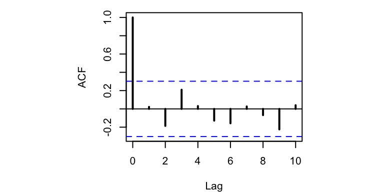

Figure 9.6: Autocorrelation plot of the forecast errors (innovations) for the DLM specified in Equations (9.19)–(9.21). Horizontal blue lines define the upper and lower 95% confidence intervals.

The ACF plot (Figure 9.6) shows no significant autocorrelation in the innovations at lags 1–10, so it looks like both of our model assumptions have indeed been met.