13.1 Linear regression
We’ll start with the simplest time series model possible: linear regression with only an intercept, so that the predicted values of all observations are the same. There are several ways we can write this equation. First, the predicted values can be written as \(E[Y_{t}] = \beta x\), where \(x=1\). Assuming that the residuals are normally distributed, the model linking our predictions to observed data is written as \[y_t = \beta x + e_{t}, e_{t} \sim N(0,\sigma), x=1\]
An equivalent way to think about this model is that instead of the residuals as normally distributed with mean zero, we can think of the data \(y_t\) as being drawn from a normal distribution with a mean of the intercept, and the same residual standard deviation: \[Y_t \sim N(E[Y_{t}],\sigma)\] Remember that in linear regression models, the residual error is interpreted as independent and identically distributed observation error.
To run this model using our package, we’ll need to specify the response and predictor variables. The covariate matrix with an intercept only is a matrix of 1s. To double check, you could always look at
x <- model.matrix(lm(Temp ~ 1))Fitting the model using our function is done with this code,
lm_intercept <- atsar::fit_stan(y = as.numeric(Temp), x = rep(1,
    length(Temp)), model_name = "regression")
Coarse summaries of stanfit objects can be examined by typing one of the following
lm_intercept
# this is huge
summary(lm_intercept)
But to get more detailed output for each parameter, you have to use the extract() function,
pars <- rstan::extract(lm_intercept)
names(pars)
[1] "beta" "sigma" "pred" "log_lik" "lp__" extract() will return the draws from the posterior for your parameters and any derived variables specified in your stan code. In this case, our model is
\[y_t = \beta \times 1 + e_t, e_t \sim N(0,\sigma)\]
so our estimated parameters are \(\beta\) and \(\sigma\). Our stan code computed the derived variables: predicted \(y_t\) which is \(\hat{y}_t = \beta \times 1\) and the log-likelihood. lp__ is the log posterior which is automatically returned.
We can then make basic plots or summaries of each of these parameters,
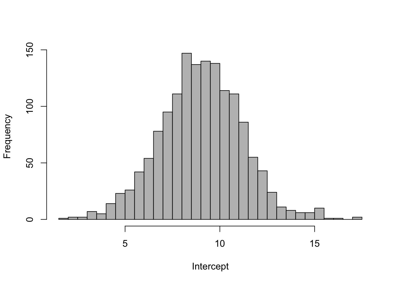
hist(pars$beta, 40, col = "grey", xlab = "Intercept", main = "")
quantile(pars$beta, c(0.025, 0.5, 0.975)) 2.5% 50% 97.5%
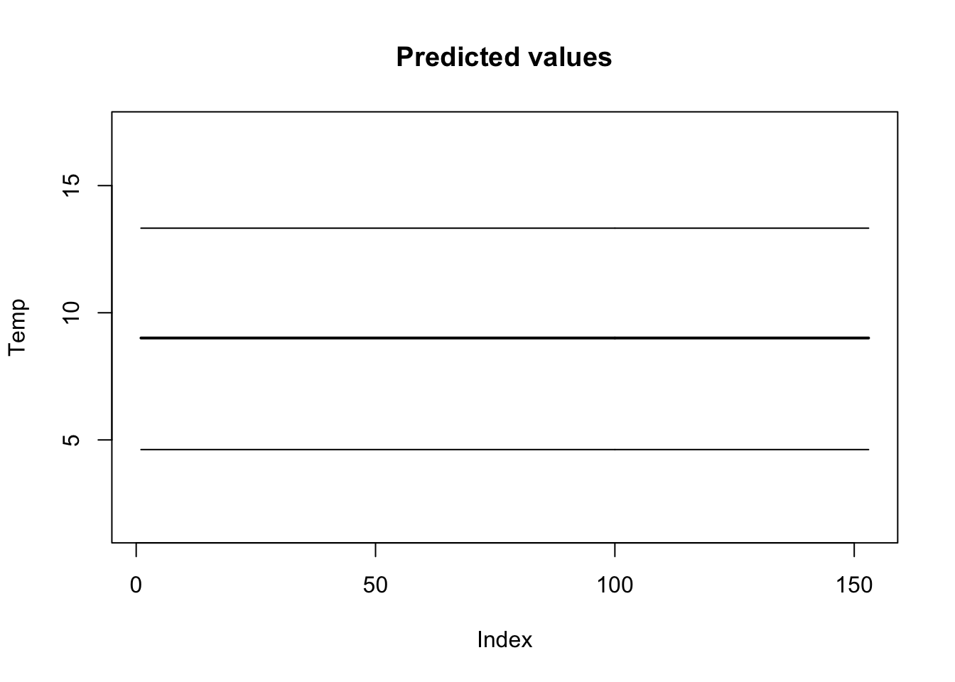
4.620617 9.016637 13.326209 One of the other useful things we can do is look at the predicted values of our model (\(\hat{y}_t=\beta \times 1\)) and overlay the data. The predicted values are pars$pred.
plot(apply(pars$pred, 2, mean), main = "Predicted values", lwd = 2,
    ylab = "Temp", ylim = c(min(pars$pred), max(pars$pred)),
    type = "l")
lines(apply(pars$pred, 2, quantile, 0.025))
lines(apply(pars$pred, 2, quantile, 0.975))
points(Temp, col = "red")
Figure 13.1: Data and predicted values for the linear regression model.
13.1.1 Burn-in and thinning
To illustrate the effects of the burn-in/warmup period and thinning, we can re-run the above model, but for just 1 MCMC chain (the default is 3).
lm_intercept <- atsar::fit_stan(y = Temp, x = rep(1, length(Temp)),
    model_name = "regression", mcmc_list = list(n_mcmc = 1000,
        n_burn = 1, n_chain = 1, n_thin = 1))
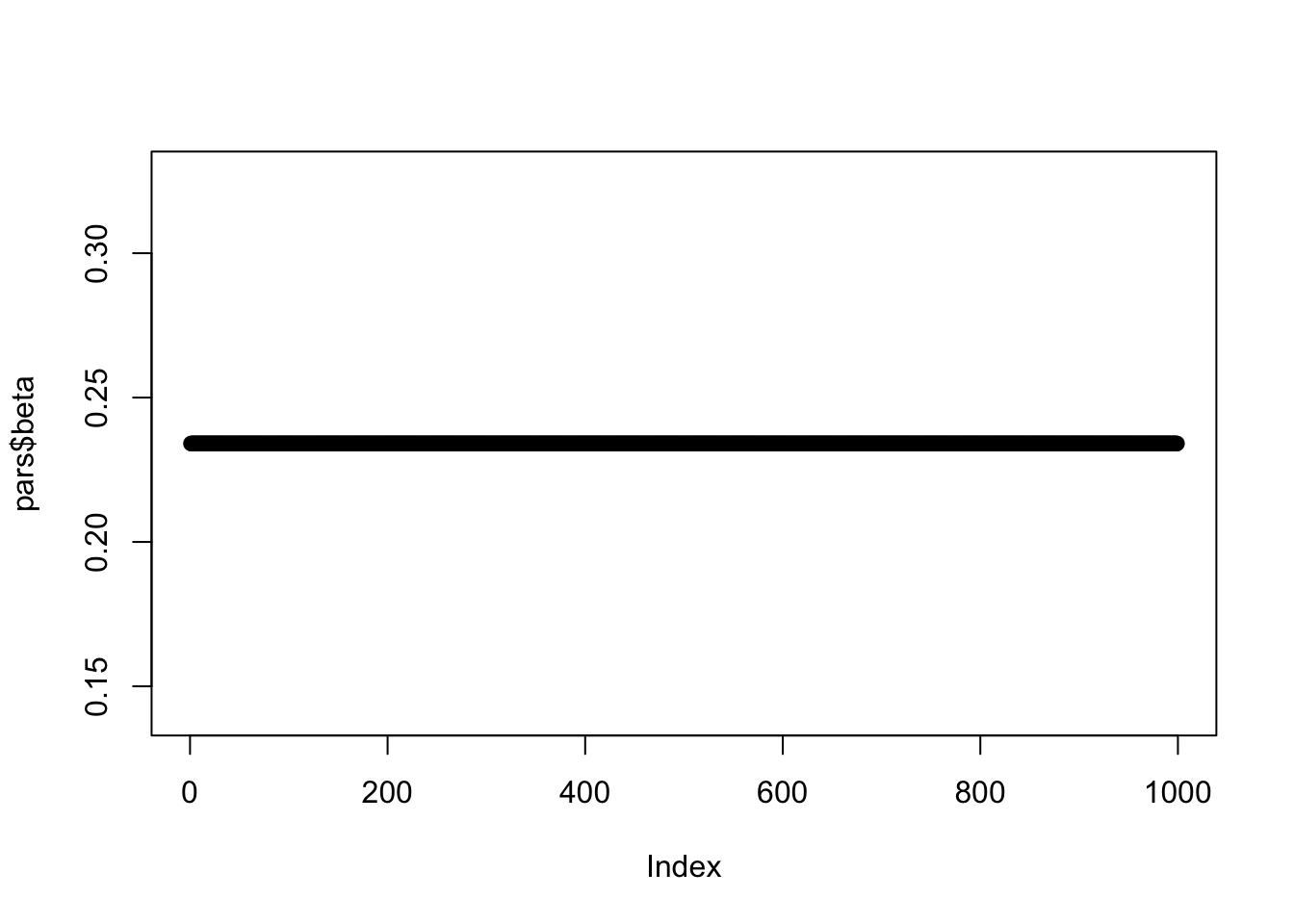
Here is a plot of the time series of beta with one chain and no burn-in. Based on visual inspection, when does the chain converge?
pars <- rstan::extract(lm_intercept)
plot(pars$beta)
Figure 13.2: A time series of our posterior draws using one chain and no burn-in.