4.7 Autoregressive (AR) models

Autoregressive models of order $p$, abbreviated AR($p$), are commonly used in time series analyses. In particular, AR(1) models (and their multivariate extensions) see considerable use in ecology as we will see later in the course. Recall from lecture that an AR($p$) model is written as

\[\begin{equation} (\#eq:defnAR.p.coef) x_t = \phi_1 x_{t-1} + \phi_2 x_{t-2} + \dots + \phi_p x_{t-p} + w_t, \end{equation}\]

where $\{w_t\}$ is a white noise sequence with zero mean and some variance $\sigma^2$. For our purposes we usually assume that $w_t \sim \text{N}(0,q)$. Note that the random walk in Equation (4.18) is a special case of an AR(1) model where $\phi_1=1$ and $\phi_k=0$ for $k \geq 2$.

4.7.1 Simulating an AR($p$) process

Although we could simulate an AR($p$) process in R using a for loop just as we did for a random walk, it’s much easier with the function arima.sim(), which works for all forms and subsets of ARIMA models. To do so, remember that the AR in ARIMA stands for “autoregressive,” the I for “integrated,” and the MA for “moving-average”; we specify the order of ARIMA models as $p,d,q$. So, for example, we would specify an AR(2) model as ARIMA(2,0,0), or an MA(1) model as ARIMA(0,0,1). If we had an ARMA(3,1) model that we applied to data that had been twice-differenced, then we would have an ARIMA(3,2,1) model.

arima.sim() will accept many arguments, but we are interested primarily in three of them (type ?arima.sim to learn more):

n: the length of desired time series
model: a list with the following elements:

order: a vector of length 3 containing the ARIMA($p,d,q$) order
ar: a vector of length $p$ containing the AR($p$) coefficients
ma: a vector of length $q$ containing the MA($q$) coefficients

sd: the standard deviation of the Gaussian errors

Note that you can omit the ma element entirely if you have an AR($p$) model, or omit the ar element if you have an MA($q$) model. If you omit the sd element, arima.sim() will assume you want normally distributed errors with SD = 1. Also note that you can pass arima.sim() your own time series of random errors or the name of a function that will generate the errors (e.g., you could use rpois() if you wanted a model with Poisson errors). Type ?arima.sim for more details.

Let’s begin by simulating some AR(1) models and comparing their behavior. First, let’s choose models with contrasting AR coefficients. Recall that in order for an AR(1) model to be stationary, $\phi < \lvert 1 \rvert$, so we’ll try 0.1 and 0.9. We’ll again set the random number seed so we will get the same answers.

set.seed(456)
## list description for AR(1) model with small coef
AR_sm <- list(order = c(1, 0, 0), ar = 0.1)
## list description for AR(1) model with large coef
AR_lg <- list(order = c(1, 0, 0), ar = 0.9)
## simulate AR(1)
AR1_sm <- arima.sim(n = 50, model = AR_sm, sd = 0.1)
AR1_lg <- arima.sim(n = 50, model = AR_lg, sd = 0.1)

Now let’s plot the 2 simulated series.

## setup plot region
par(mfrow = c(1, 2))
## get y-limits for common plots
ylm <- c(min(AR1_sm, AR1_lg), max(AR1_sm, AR1_lg))
## plot the ts
plot.ts(AR1_sm, ylim = ylm, ylab = expression(italic(x)[italic(t)]), 
    main = expression(paste(phi, " = 0.1")))
plot.ts(AR1_lg, ylim = ylm, ylab = expression(italic(x)[italic(t)]), 
    main = expression(paste(phi, " = 0.9")))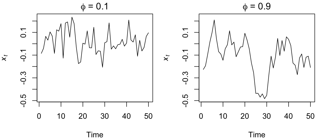

$Time series of simulated AR(1) processes with $\phi=0.1$ (left) and $\phi=0.9$ (right).$

Figure 4.22: Time series of simulated AR(1) processes with $\phi=0.1$ (left) and $\phi=0.9$ (right).

What do you notice about the two plots in Figure 4.22? It looks like the time series with the smaller AR coefficient is more “choppy” and seems to stay closer to 0 whereas the time series with the larger AR coefficient appears to wander around more. Remember that as the coefficient in an AR(1) model goes to 0, the model approaches a WN sequence, which is stationary in both the mean and variance. As the coefficient goes to 1, however, the model approaches a random walk, which is not stationary in either the mean or variance.

Next, let’s generate two AR(1) models that have the same magnitude coeficient, but opposite signs, and compare their behavior.

set.seed(123)
## list description for AR(1) model with small coef
AR_pos <- list(order = c(1, 0, 0), ar = 0.5)
## list description for AR(1) model with large coef
AR_neg <- list(order = c(1, 0, 0), ar = -0.5)
## simulate AR(1)
AR1_pos <- arima.sim(n = 50, model = AR_pos, sd = 0.1)
AR1_neg <- arima.sim(n = 50, model = AR_neg, sd = 0.1)

OK, let’s plot the 2 simulated series.

## setup plot region
par(mfrow = c(1, 2))
## get y-limits for common plots
ylm <- c(min(AR1_pos, AR1_neg), max(AR1_pos, AR1_neg))
## plot the ts
plot.ts(AR1_pos, ylim = ylm, ylab = expression(italic(x)[italic(t)]), 
    main = expression(paste(phi[1], " = 0.5")))
plot.ts(AR1_neg, ylab = expression(italic(x)[italic(t)]), main = expression(paste(phi[1], 
    " = -0.5")))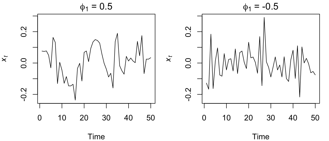

$Time series of simulated AR(1) processes with $\phi_1=0.5$ (left) and $\phi_1=-0.5$ (right).$

Figure 4.23: Time series of simulated AR(1) processes with $\phi_1=0.5$ (left) and $\phi_1=-0.5$ (right).

Now it appears like both time series vary around the mean by about the same amount, but the model with the negative coefficient produces a much more “sawtooth” time series. It turns out that any AR(1) model with $-1<\phi<0$ will exhibit the 2-point oscillation you see here.

We can simulate higher order AR($p$) models in the same manner, but care must be exercised when choosing a set of coefficients that result in a stationary model or else arima.sim() will fail and report an error. For example, an AR(2) model with both coefficients equal to 0.5 is not stationary, and therefore this function call will not work:

arima.sim(n = 100, model = list(order(2, 0, 0), ar = c(0.5, 0.5)))

If you try, R will respond that the “'ar' part of model is not stationary.”

4.7.2 Correlation structure of AR($p$) processes

Let’s review what we learned in lecture about the general behavior of the ACF and PACF for AR($p$) models. To do so, we’ll simulate four stationary AR($p$) models of increasing order $p$ and then examine their ACF’s and PACF’s. Let’s use a really big $n$ so as to make them “pure,” which will provide a much better estimate of the correlation structure.

set.seed(123)
## the 4 AR coefficients
AR_p_coef <- c(0.7, 0.2, -0.1, -0.3)
## empty list for storing models
AR_mods <- list()
## loop over orders of p
for (p in 1:4) {
    ## assume sd = 1, so not specified
    AR_mods[[p]] <- arima.sim(n = 10000, list(ar = AR_p_coef[1:p]))
}

Now that we have our four AR($p$) models, lets look at plots of the time series, ACF’s, and PACF’s.

## set up plot region
par(mfrow = c(4, 3))
## loop over orders of p
for (p in 1:4) {
    plot.ts(AR_mods[[p]][1:50], ylab = paste("AR(", p, ")", sep = ""))
    acf(AR_mods[[p]], lag.max = 12)
    pacf(AR_mods[[p]], lag.max = 12, ylab = "PACF")
}

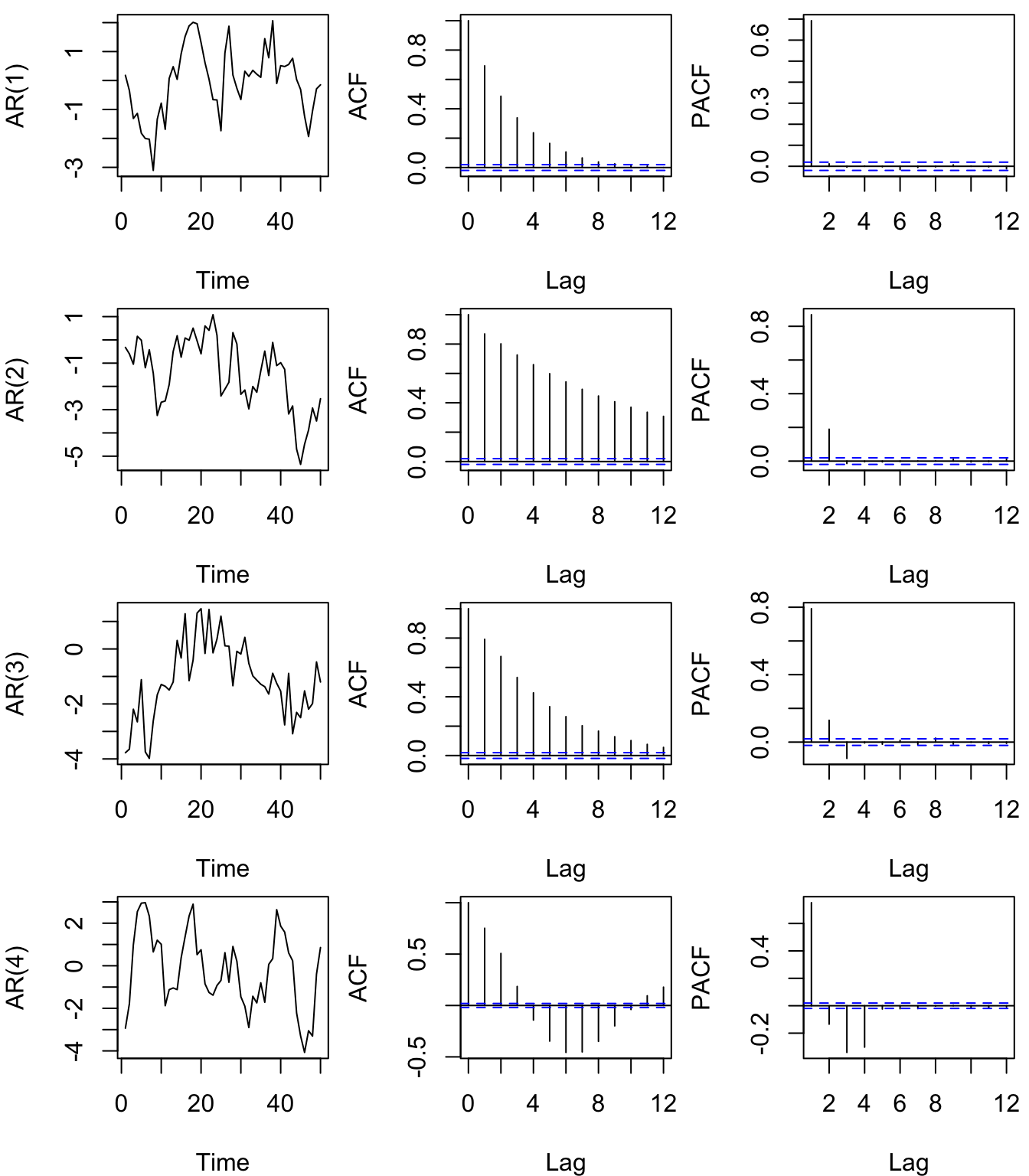
$Time series of simulated AR($p$) processes (left column) of increasing orders from 1-4 (rows) with their associated ACF’s (center column) and PACF’s (right column). Note that only the first 50 values of $x_t$ are plotted.$

Figure 4.24: Time series of simulated AR($p$) processes (left column) of increasing orders from 1-4 (rows) with their associated ACF’s (center column) and PACF’s (right column). Note that only the first 50 values of $x_t$ are plotted.

As we saw in lecture and is evident from our examples shown in Figure 4.24, the ACF for an AR($p$) process tails off toward zero very slowly, but the PACF goes to zero for lags > $p$. This is an important diagnostic tool when trying to identify the order of $p$ in ARMA($p,q$) models.

Applied Time Series Analysis for Fisheries and Environmental Sciences

4.7 Autoregressive (AR) models

4.7.1 Simulating an AR(\(p\)) process

4.7.2 Correlation structure of AR(\(p\)) processes