6.7 Fitting with Stan
Let’s fit the same model with Stan using the rstan package. If you have not already, you will need to install the rstan package. This package depends on a number of other packages which should install automatically when you install rstan.
library(datasets)
library(rstan)
y <- as.vector(Nile)
First we write the model. We could write this to a file (recommended), but for this example, we write as a character object. Though the syntax is different from the JAGS code, it has many similarities. Note, unlike the JAGS, the Stan does not allow any NAs in your data. Thus we have to specify the location of the NAs in our data. The Nile data does not have NAs, but we want to write the code so it would work even if there were NAs.
scode <- "
data {
  int<lower=0> TT;
  int<lower=0> n_pos; // number of non-NA values
  int<lower=0> indx_pos[n_pos]; // index of the non-NA values
  vector[n_pos] y;
}
parameters {
  real x0;
  real u;
  vector[TT] pro_dev;
  real<lower=0> sd_q;
  real<lower=0> sd_r;
}
transformed parameters {
  vector[TT] x;
  x[1] = x0 + u + pro_dev[1];
  for(i in 2:TT) {
    x[i] = x[i-1] + u + pro_dev[i];
  }
}
model {
  x0 ~ normal(y[1],10);
  u ~ normal(0,2);
  sd_q ~ cauchy(0,5);
  sd_r ~ cauchy(0,5);
  pro_dev ~ normal(0, sd_q);
  for(i in 1:n_pos){
    y[i] ~ normal(x[indx_pos[i]], sd_r);
  }
}
generated quantities {
  vector[n_pos] log_lik;
  for (i in 1:n_pos) log_lik[i] = normal_lpdf(y[i] | x[indx_pos[i]], sd_r);
}
"
Then we call stan() and pass in the data, names of parameter we wish to have returned, and information on number of chains, samples (iter), and thinning. The output is verbose (hidden here) and may have some warnings.
# We pass in the non-NA ys as vector
ypos <- y[!is.na(y)]
n_pos <- sum(!is.na(y))  # number on non-NA ys
indx_pos <- which(!is.na(y))  # index on the non-NAs
mod <- rstan::stan(model_code = scode, data = list(y = ypos,
    TT = length(y), n_pos = n_pos, indx_pos = indx_pos), pars = c("sd_q",
    "x", "sd_r", "u", "x0"), chains = 3, iter = 1000, thin = 1)
We use extract() to extract the parameters from the fitted model and we can plot. The estimated level is x and we will plot that with the 95% credible intervals.
pars <- rstan::extract(mod)
pred_mean <- apply(pars$x, 2, mean)
pred_lo <- apply(pars$x, 2, quantile, 0.025)
pred_hi <- apply(pars$x, 2, quantile, 0.975)
plot(pred_mean, type = "l", lwd = 3, ylim = range(c(pred_mean,
    pred_lo, pred_hi)), ylab = "Nile River Level")
lines(pred_lo)
lines(pred_hi)
points(y, col = "blue")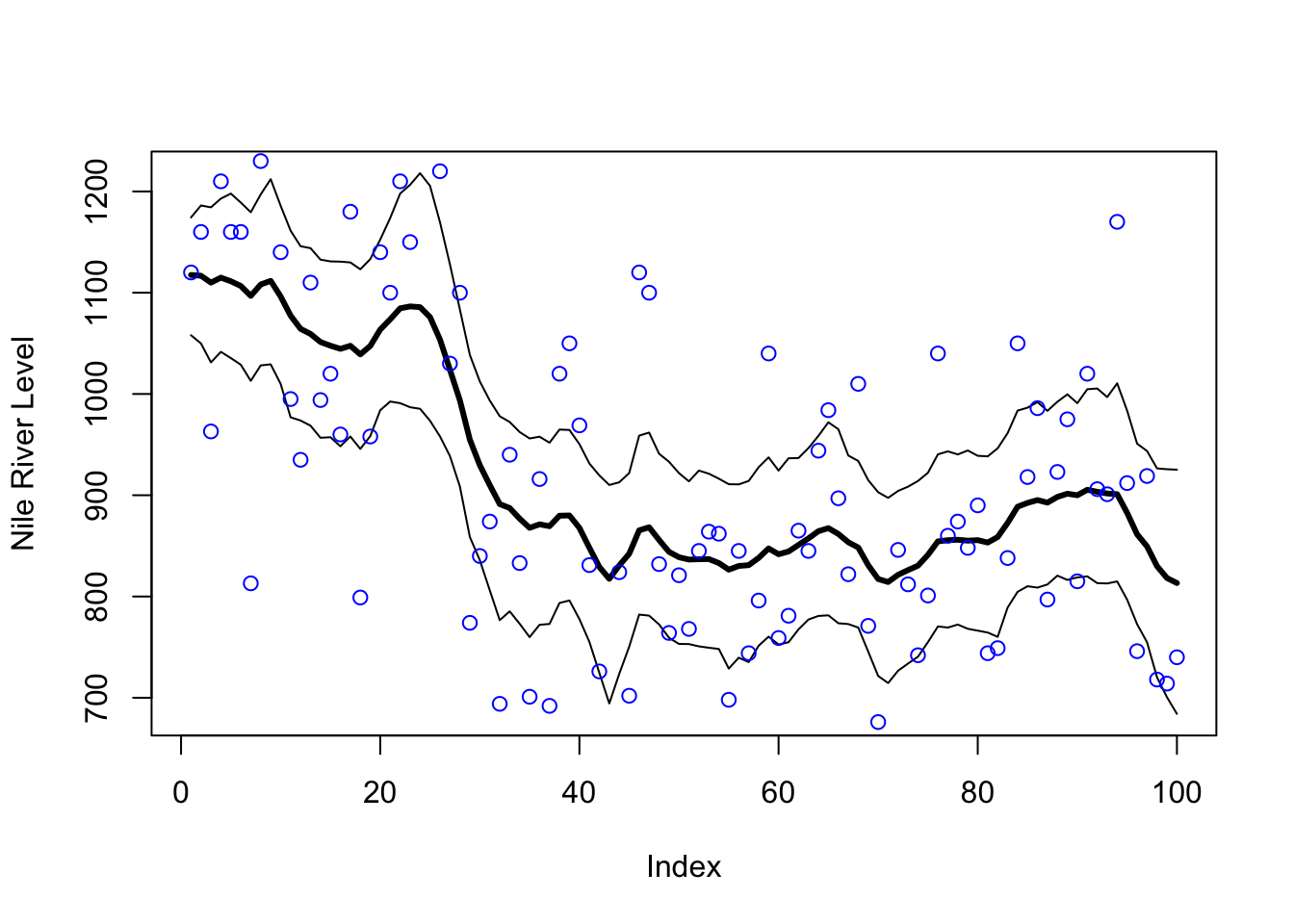
Figure 6.8: Estimated level and 95 percent credible intervals. Blue dots are the actual Nile River levels.
Here is a ggplot() version of the plot.
library(ggplot2)
nile <- data.frame(y = y, year = 1871:1970)
h <- ggplot(nile, aes(year))
h + geom_ribbon(aes(ymin = pred_lo, ymax = pred_hi), fill = "grey70") +
    geom_line(aes(y = pred_mean), size = 1) + geom_point(aes(y = y),
    color = "blue") + labs(y = "Nile River level")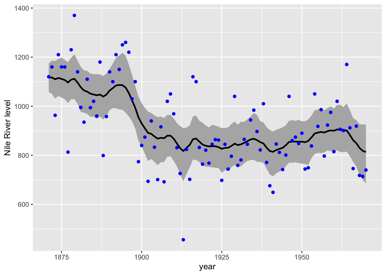
Figure 6.9: Estimated level and 95 percent credible intervals
We can plot the histogram of the samples against the values estimated via maximum likelihood.
par(mfrow = c(2, 2))
hist(pars$x0)
abline(v = coef(kem.3)$x0, col = "red")
hist(pars$u)
abline(v = coef(kem.3)$U, col = "red")
hist(log(pars$sd_q^2))
abline(v = log(coef(kem.3)$Q), col = "red")
hist(log(pars$sd_r^2))
abline(v = log(coef(kem.3)$R), col = "red")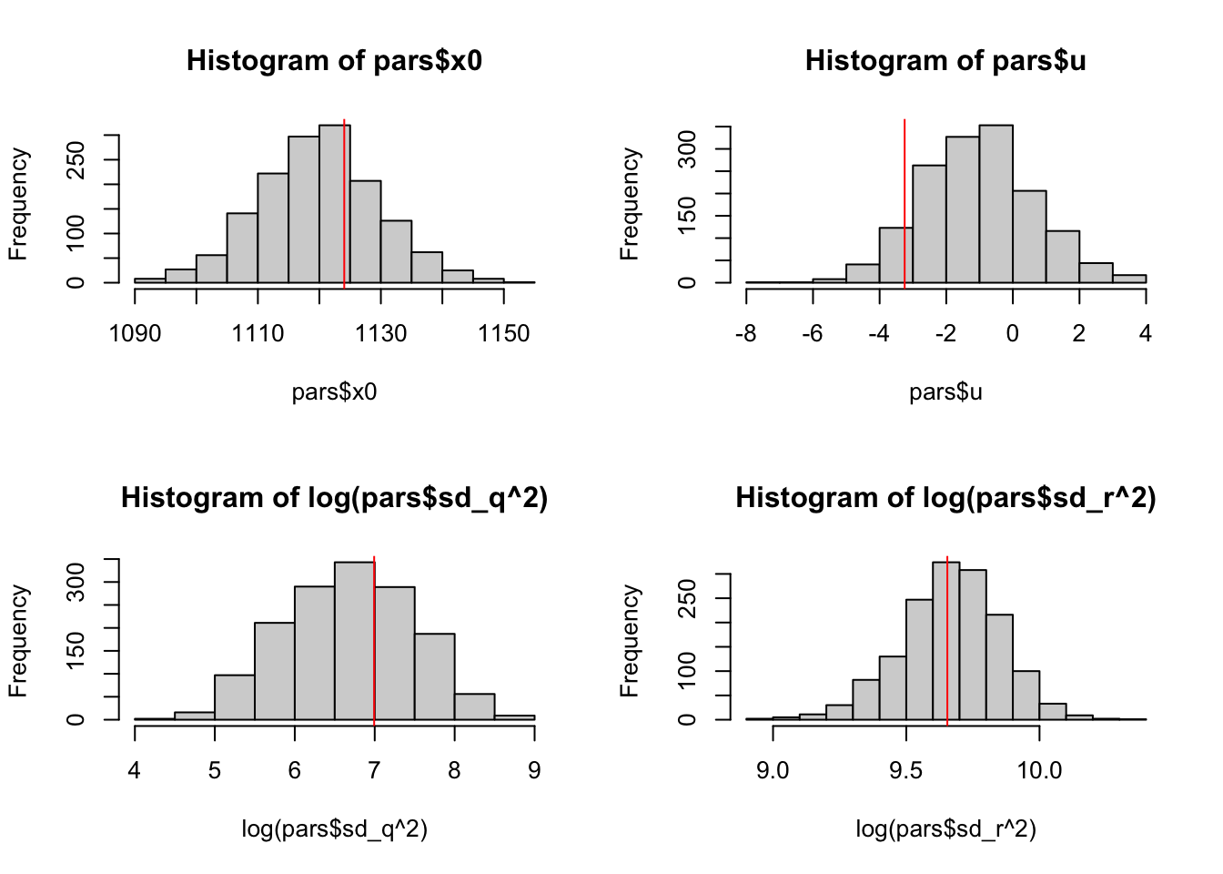
Figure 6.10: Histogram of the parameter samples versus the estimate (red line) from maximum likelihood.