7.10 Fitting a MARSS model with Stan

Let’s fit the same model as in Section 7.9 with Stan using the rstan package. If you have not already, you will need to install the rstan package. This package depends on a number of other packages which should install automatically when you install rstan.

First we write the model. We could write this to a file (recommended), but for this example, we write as a character object. Though the syntax is different from the JAGS code, it has many similarities. Note that Stan does not allow missing values in the data, thus we need to pass in only the non-missing values along with the row and column indices of those values. The latter is so we can match them to the appropriate state (\(x\)) values.

scode <- "
data {
  int<lower=0> TT; // length of ts
  int<lower=0> N; // num of ts; rows of y
  int<lower=0> n_pos; // number of non-NA values in y
  int<lower=0> col_indx_pos[n_pos]; // col index of non-NA vals
  int<lower=0> row_indx_pos[n_pos]; // row index of non-NA vals
  vector[n_pos] y;
}
parameters {
  vector[N] x0; // initial states
  real u;
  vector[N] pro_dev[TT]; // refed as pro_dev[TT,N]
  real<lower=0> sd_q;
  real<lower=0> sd_r[N]; // obs variances are different
}
transformed parameters {
  vector[N] x[TT]; // refed as x[TT,N]
  for(i in 1:N){
    x[1,i] = x0[i] + u + pro_dev[1,i];
    for(t in 2:TT) {
      x[t,i] = x[t-1,i] + u + pro_dev[t,i];
    }
  }
}
model {
  sd_q ~ cauchy(0,5);
  for(i in 1:N){
    x0[i] ~ normal(y[i],10); // assume no missing y[1]
    sd_r[i] ~ cauchy(0,5);
    for(t in 1:TT){
    pro_dev[t,i] ~ normal(0, sd_q);
    }
  }
  u ~ normal(0,2);
  for(i in 1:n_pos){
    y[i] ~ normal(x[col_indx_pos[i], row_indx_pos[i]], sd_r[row_indx_pos[i]]);
  }
}
generated quantities {
  vector[n_pos] log_lik;
  for (n in 1:n_pos) log_lik[n] = normal_lpdf(y[n] | x[col_indx_pos[n], row_indx_pos[n]], sd_r[row_indx_pos[n]]);
}
"

Then we call stan() and pass in the data, names of parameter we wish to have returned, and information on number of chains, samples (iter), and thinning. The output is verbose (hidden here) and may have some warnings.

ypos <- Y[!is.na(Y)]
n_pos <- length(ypos)  # number on non-NA ys
indx_pos <- which(!is.na(Y), arr.ind = TRUE)  # index on the non-NAs
col_indx_pos <- as.vector(indx_pos[, "col"])
row_indx_pos <- as.vector(indx_pos[, "row"])
mod <- rstan::stan(model_code = scode, data = list(y = ypos, 
    TT = ncol(Y), N = nrow(Y), n_pos = n_pos, col_indx_pos = col_indx_pos, 
    row_indx_pos = row_indx_pos), pars = c("sd_q", "x", "sd_r", 
    "u", "x0"), chains = 3, iter = 1000, thin = 1)

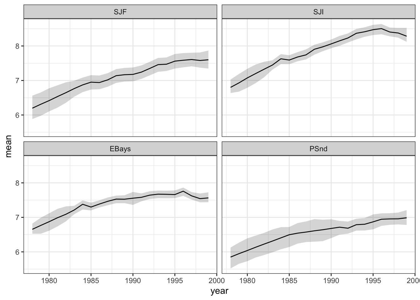
We use extract() to extract the parameters from the fitted model and then the means and 95% credible intervals.

pars <- rstan::extract(mod)
means <- apply(pars$x, c(2, 3), mean)
upperCI <- apply(pars$x, c(2, 3), quantile, 0.975)
lowerCI <- apply(pars$x, c(2, 3), quantile, 0.025)
colnames(means) <- colnames(upperCI) <- colnames(lowerCI) <- rownames(Y)

No id variables; using all as measure variables
No id variables; using all as measure variables
No id variables; using all as measure variables

Figure 7.7: Estimated level and 95 percent credible intervals.