9.3 Stochastic level models

The most simple DLM is a stochastic level model, where the level is a random walk without drift, and this level is observed with error. We will write it first in using regression notation where the intercept is \(\alpha\) and then in MARSS notation. In the latter, \(\alpha_t=x_t\).

\[\begin{equation} \begin{gathered} \tag{9.5} y_t = \alpha_t + e_t \\ \alpha_t = \alpha_{t-1} + w_t \\ \Downarrow \\ y_t = x_t + v_t \\ x_t = x_{t-1} + w_t \end{gathered} \end{equation}\]

Using this model, we can model the Nile River level and fit the model using MARSS().

## load Nile flow data
data(Nile, package = "datasets")

## define model list
mod_list <- list(B = "identity", U = "zero", Q = matrix("q"), 
    Z = "identity", A = matrix("a"), R = matrix("r"))

## fit the model with MARSS
fit <- MARSS(matrix(Nile, nrow = 1), mod_list)

Success! abstol and log-log tests passed at 82 iterations.
Alert: conv.test.slope.tol is 0.5.
Test with smaller values (<0.1) to ensure convergence.

MARSS fit is
Estimation method: kem 
Convergence test: conv.test.slope.tol = 0.5, abstol = 0.001
Estimation converged in 82 iterations. 
Log-likelihood: -637.7569 
AIC: 1283.514   AICc: 1283.935   
 
       Estimate
A.a      -0.338
R.r   15135.796
Q.q    1381.153
x0.x0  1111.791
Initial states (x0) defined at t=0

Standard errors have not been calculated. 
Use MARSSparamCIs to compute CIs and bias estimates.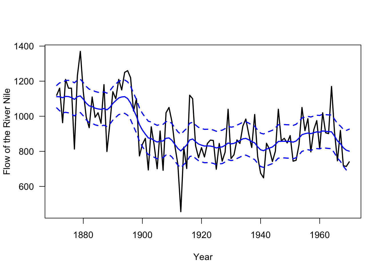

9.3.1 Stochastic level with drift

We can add a drift term to the level model to allow the level to tend upward or downward with a deterministic rate \(\eta\). This is a random walk with bias.

\[\begin{equation} \begin{gathered} \tag{9.6} y_t = \alpha_t + e_t \\ \alpha_t = \alpha_{t-1} + \eta + w_t \\ \Downarrow \\ y_t = x_t + v_t \\ x_t = x_{t-1} + u + w_t \end{gathered} \end{equation}\]

We can allow that the drift term \(\eta\) evolves over time along with the level. In this case, \(\eta\) is modeled as a random walk along with \(\alpha\). This model is

\[\begin{equation} \begin{gathered} \tag{9.7} y_t = \alpha_t + e_t \\ \alpha_t = \alpha_{t-1} + \eta_{t-1} + w_{\alpha,t} \\ \eta_t = \eta_{t-1} + w_{\eta,t} \end{gathered} \end{equation}\] Equation (9.7) can be written in matrix form as: \[\begin{equation} \begin{gathered} \tag{9.8} y_t = \begin{bmatrix}1&0\end{bmatrix}\begin{bmatrix} \alpha \\ \eta \end{bmatrix}_t + v_t \\ \begin{bmatrix} \alpha \\ \eta \end{bmatrix}_t = \begin{bmatrix} 1 & 1 \\ 0 & 1 \end{bmatrix}\begin{bmatrix} \alpha \\ \eta \end{bmatrix}_{t-1} + \begin{bmatrix} w_{\alpha} \\ w_{\eta} \end{bmatrix}_t \end{gathered} \end{equation}\] Equation (9.8) is a MARSS model.

\[\begin{equation} y_t = \mathbf{Z}\mathbf{x}_t + v_t \\ \mathbf{x}_t = \mathbf{B}\mathbf{x}_{t-1} + \mathbf{w}_t \end{equation}\]

where \(\mathbf{B}=\begin{bmatrix} 1 & 1 \\ 0 & 1\end{bmatrix}\), \(\mathbf{x}=\begin{bmatrix}\alpha \\ \eta\end{bmatrix}\) and \(\mathbf{Z}=\begin{bmatrix}1&0\end{bmatrix}\).

See Section 6.2 for more discussion of stochastic level models and Section @ref() to see how to fit this model with the StructTS(sec-uss-the-structts-function) function in the stats package.