10.5 Lake Washington phytoplankton data
For this exercise, we will use the Lake Washington phytoplankton data contained in the MARSS package. Let’s begin by reading in the monthly values for all of the data, including metabolism, chemistry, and climate.
## load the data (there are 3 datasets contained here)
data(lakeWAplankton, package = "MARSS")
## we want lakeWAplanktonTrans, which has been transformed
## so the 0s are replaced with NAs and the data z-scored
all_dat <- lakeWAplanktonTrans
## use only the 10 years from 1980-1989
yr_frst <- 1980
yr_last <- 1989
plank_dat <- all_dat[all_dat[, "Year"] >= yr_frst & all_dat[,
    "Year"] <= yr_last, ]
## create vector of phytoplankton group names
phytoplankton <- c("Cryptomonas", "Diatoms", "Greens", "Unicells",
    "Other.algae")
## get only the phytoplankton
dat_1980 <- plank_dat[, phytoplankton]
Next, we transpose the data matrix and calculate the number of time series and their length.
## transpose data so time goes across columns
dat_1980 <- t(dat_1980)
## get number of time series
N_ts <- dim(dat_1980)[1]
## get length of time series
TT <- dim(dat_1980)[2]
It will be easier to estimate the real parameters of interest if we de-mean the data, so let’s do that.
y_bar <- apply(dat_1980, 1, mean, na.rm = TRUE)
dat <- dat_1980 - y_bar
rownames(dat) <- rownames(dat_1980)
10.5.1 Plots of the data
Here are time series plots of all five phytoplankton functional groups.
spp <- rownames(dat_1980)
clr <- c("brown", "blue", "darkgreen", "darkred", "purple")
cnt <- 1
par(mfrow = c(N_ts, 1), mai = c(0.5, 0.7, 0.1, 0.1), omi = c(0,
    0, 0, 0))
for (i in spp) {
    plot(dat[i, ], xlab = "", ylab = "Abundance index", bty = "L",
        xaxt = "n", pch = 16, col = clr[cnt], type = "b")
    axis(1, 12 * (0:dim(dat_1980)[2]) + 1, yr_frst + 0:dim(dat_1980)[2])
    title(i)
    cnt <- cnt + 1
}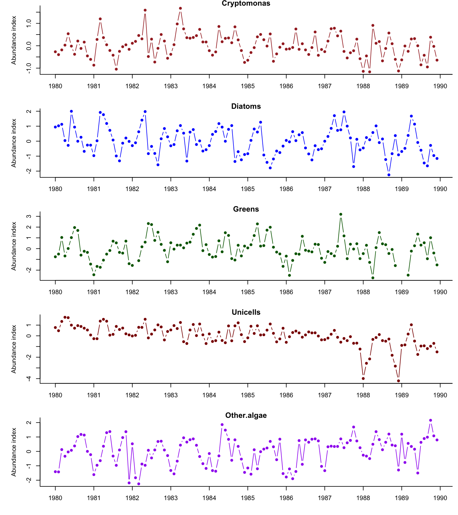
Figure 10.1: Demeaned time series of Lake Washington phytoplankton.