5.7 Estimating ARMA parameters

Let’s start with fitting to simulated data.

5.7.1 AR(2) data

Simulate AR(2) data and add a mean level so that the data are not mean 0.

\[\begin{equation} \begin{gathered} x_t = 0.8 x_{t-1} + 0.1 x_{t-2} + e_t\\ y_t = x_t + m \end{gathered} \end{equation}\]

m <- 1
ar2 <- arima.sim(n = 1000, model = list(ar = c(0.8, 0.1))) + 
    m

To see info on arima.sim(), type ?arima.sim.

5.7.2 Fit with `Arima()`

Fit an ARMA(2) with level to the data.

forecast::Arima(ar2, order = c(2, 0, 0), include.constant = TRUE)

Series: ar2 
ARIMA(2,0,0) with non-zero mean 

Coefficients:
         ar1     ar2    mean
      0.7684  0.1387  0.9561
s.e.  0.0314  0.0314  0.3332

sigma^2 estimated as 0.9832:  log likelihood=-1409.77
AIC=2827.54   AICc=2827.58   BIC=2847.17

Note, the model being fit by Arima() is not this model

\[\begin{equation} y_t = m + 0.8 y_{t-1} + 0.1 y_{t-2} + e_t \end{equation}\]

It is this model:

\[\begin{equation} (y_t - m) = 0.8 (y_{t-1}-m) + 0.1 (y_{t-2}-m)+ e_t \end{equation}\]

or as written above: \[\begin{equation} \begin{gathered} x_t = 0.8 x_{t-1} + 0.1 x_{t-2} + e_t\\ y_t = x_t + m \end{gathered} \end{equation}\]

We could also use arima() to fit to the data.

arima(ar2, order = c(2, 0, 0), include.mean = TRUE)

Warning in arima(ar2, order = c(2, 0, 0), include.mean = TRUE): possible
convergence problem: optim gave code = 1


Call:
arima(x = ar2, order = c(2, 0, 0), include.mean = TRUE)

Coefficients:
         ar1     ar2  intercept
      0.7684  0.1387     0.9561
s.e.  0.0314  0.0314     0.3332

sigma^2 estimated as 0.9802:  log likelihood = -1409.77,  aic = 2827.54

However we will not be using arima() directly because for if we have differenced data, it will not allow us to include and estimated mean level. Unless we have transformed our differenced data in a way that ensures it is mean zero, then we want to include a mean.

Try increasing the length of the simulated data (from 100 to 1000 say) and see how that affects your parameter estimates. Run the simulation a few times.

5.7.3 AR(1) simulated data

ar1 <- arima.sim(n = 100, model = list(ar = c(0.8))) + m
forecast::Arima(ar1, order = c(1, 0, 0), include.constant = TRUE)

Series: ar1 
ARIMA(1,0,0) with non-zero mean 

Coefficients:
         ar1    mean
      0.7091  0.4827
s.e.  0.0705  0.3847

sigma^2 estimated as 1.34:  log likelihood=-155.85
AIC=317.7   AICc=317.95   BIC=325.51

5.7.4 ARMA(1,2) simulated data

Simulate ARMA(1,2) \[x_t = 0.8 x_{t-1} + e_t + 0.8 e_{t-1} + 0.2 e_{t-2}\]

arma12 = arima.sim(n = 100, model = list(ar = c(0.8), ma = c(0.8, 
    0.2))) + m
forecast::Arima(arma12, order = c(1, 0, 2), include.constant = TRUE)

Series: arma12 
ARIMA(1,0,2) with non-zero mean 

Coefficients:
         ar1     ma1     ma2    mean
      0.8138  0.8599  0.1861  0.3350
s.e.  0.0646  0.1099  0.1050  0.8145

sigma^2 estimated as 0.6264:  log likelihood=-118.02
AIC=246.03   AICc=246.67   BIC=259.06

We will up the number of data points to 1000 because models with a MA component take a lot of data to estimate. Models with MA(>1) are not very practical for fisheries data for that reason.

5.7.5 These functions work for data with missing values

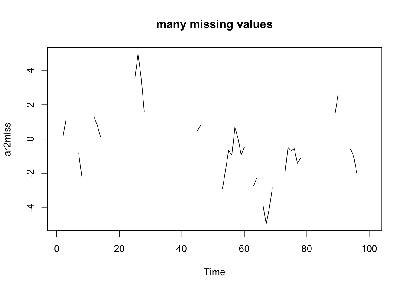
Create some AR(2) data and then add missing values (NA).

ar2miss <- arima.sim(n = 100, model = list(ar = c(0.8, 0.1)))
ar2miss[sample(100, 50)] <- NA
plot(ar2miss, type = "l")
title("many missing values")

Fit

fit <- forecast::Arima(ar2miss, order = c(2, 0, 0))
fit

Series: ar2miss 
ARIMA(2,0,0) with non-zero mean 

Coefficients:
         ar1      ar2     mean
      1.0625  -0.2203  -0.0586
s.e.  0.1555   0.1618   0.6061

sigma^2 estimated as 0.9679:  log likelihood=-79.86
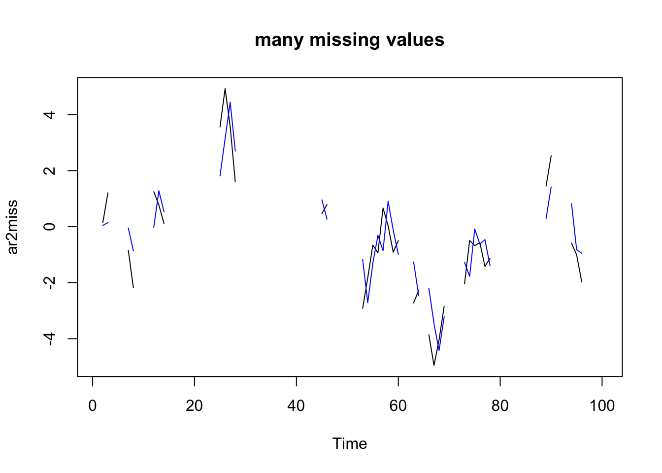
AIC=167.72   AICc=168.15   BIC=178.06

Note fitted() does not return the expected value at time \(t\). It is the expected value of \(y_t\) given the data up to time \(t-1\).

plot(ar2miss, type = "l")
title("many missing values")
lines(fitted(fit), col = "blue")

It is easy enough to get the expected value of \(y_t\) for all the missing values but we’ll learn to do that when we learn the MARSS package and can apply the Kalman Smoother in that package.