5.11 Seasonal ARIMA model

The Chinook data are monthly and start in January 1990. To make this into a ts object do

chinookts <- ts(chinook$log.metric.tons, start = c(1990, 1), 
    frequency = 12)

start is the year and month and frequency is the number of months in the year.

Use ?ts to see more examples of how to set up ts objects.

5.11.1 Plot seasonal data

plot(chinookts)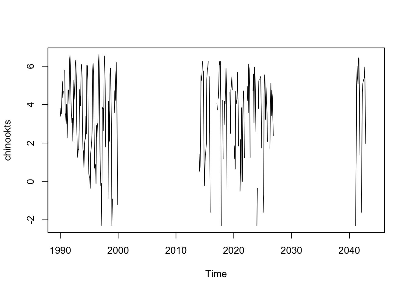

5.11.2 auto.arima() for seasonal ts

auto.arima() will recognize that our data has season and fit a seasonal ARIMA model to our data by default. Let’s define the training data up to 1998 and use 1999 as the test data.

traindat <- window(chinookts, c(1990, 10), c(1998, 12))
testdat <- window(chinookts, c(1999, 1), c(1999, 12))
fit <- forecast::auto.arima(traindat)
fit

Series: traindat 
ARIMA(1,0,0)(0,1,0)[12] with drift 

Coefficients:
         ar1    drift
      0.3676  -0.0320
s.e.  0.1335   0.0127

sigma^2 estimated as 0.8053:  log likelihood=-107.37
AIC=220.73   AICc=221.02   BIC=228.13

Use ?window to understand how subsetting a ts object works.