4  Climate Variables

library(tidyverse)
options(dplyr.summarise.inform = FALSE)

Climate Indices

See also https://psl.noaa.gov/data/atmoswrit/corr/timeseries/ and https://psl.noaa.gov/data/climateindices/list/.

I have created a dataset of seasonal climate variables from the PSL page.

Seasons are defined as:

• Winter: January, February, March
• Spring: April, May, June
• Summer: May, June, July, August
• Fall: September, October, November
• Annual: whole year

Variables:

Index	Region	Influences on Salmon	Notes
PDO (Pacific Decadal Oscillation)	North Pacific	Ocean productivity, survival of juveniles	Warm phase reduces survival in Alaska, improves in CA.
ONI (Oceanic Niño Index)	Equatorial Pacific (global effects)	Marine heatwaves, prey availability	El Niño years generally reduce survival along West Coast.
MEIv2 (Multivariate ENSO Index)	Equatorial Pacific/global	Similar to ONI but broader; marine habitat stress	Integrated index of ENSO variability; affects productivity.
PNA (Pacific-North American Pattern)	North America and North Pacific	River flows, snowpack, freshwater survival	Positive PNA linked to warmer/drier winters, lower survival.
EPO (East Pacific Oscillation)	Eastern North Pacific	Winter ocean conditions	Negative EPO can improve early marine survival conditions.
WP (Western Pacific Pattern)	Western Pacific, Eastern Asia	Atmospheric circulation affecting ocean entry timing	Alters timing and success of smolt outmigration indirectly.
CENSO (Central ENSO Index)	Central Pacific	Central Pacific ENSO variability	May modulate effects of traditional El Niño on survival.
WHWP (Western Hemisphere Warm Pool)	Atlantic and Eastern Pacific	Hurricane activity (Atlantic)	Not directly linked to salmon survival in the North Pacific.
IPOTPI (Indo-Pacific Ocean Temperature Pattern Index)	Indo-Pacific	Tropical SST variability patterns	Emerging index; indirect possible link to broad-scale climate affecting salmon.
NP (North Pacific Index)	North Pacific	Aleutian Low strength, ocean upwelling	Strong Aleutian Low (lower NP) → better salmon survival.
PACWARM (Pacific Warm Pool Index)	Equatorial Pacific	Warm pool expansion influencing ENSO events	Can modulate strength of El Niño impacts on marine survival.
GMSST (Global Mean Sea Surface Temperature)	Global Ocean	Baseline warming trend	Higher GMSST linked to long-term habitat stress.

Loading data

I have created a data frame of North Pacific climate variables from NOAA PSL. Update your atsalibrary to version 1.6 to get the climate data or load np_climate.RData from the Data_Images directory.

library(atsalibrary)
data("np_climate")
# this has seasonal and annual averages
# use ?np_climate for info
colnames(np_climate_month)

 [1] "date"    "year"    "month"   "pna"     "epo"     "wp"      "censo"  
 [8] "whwp"    "oni"     "meiv2"   "pdo"     "ipotpi"  "np"      "pacwarm"
[15] "gmsst"  

pdots <- ts(np_climate_month$pdo, freq=12, start=c(np_climate_month$year[1], 1))
plot(pdots)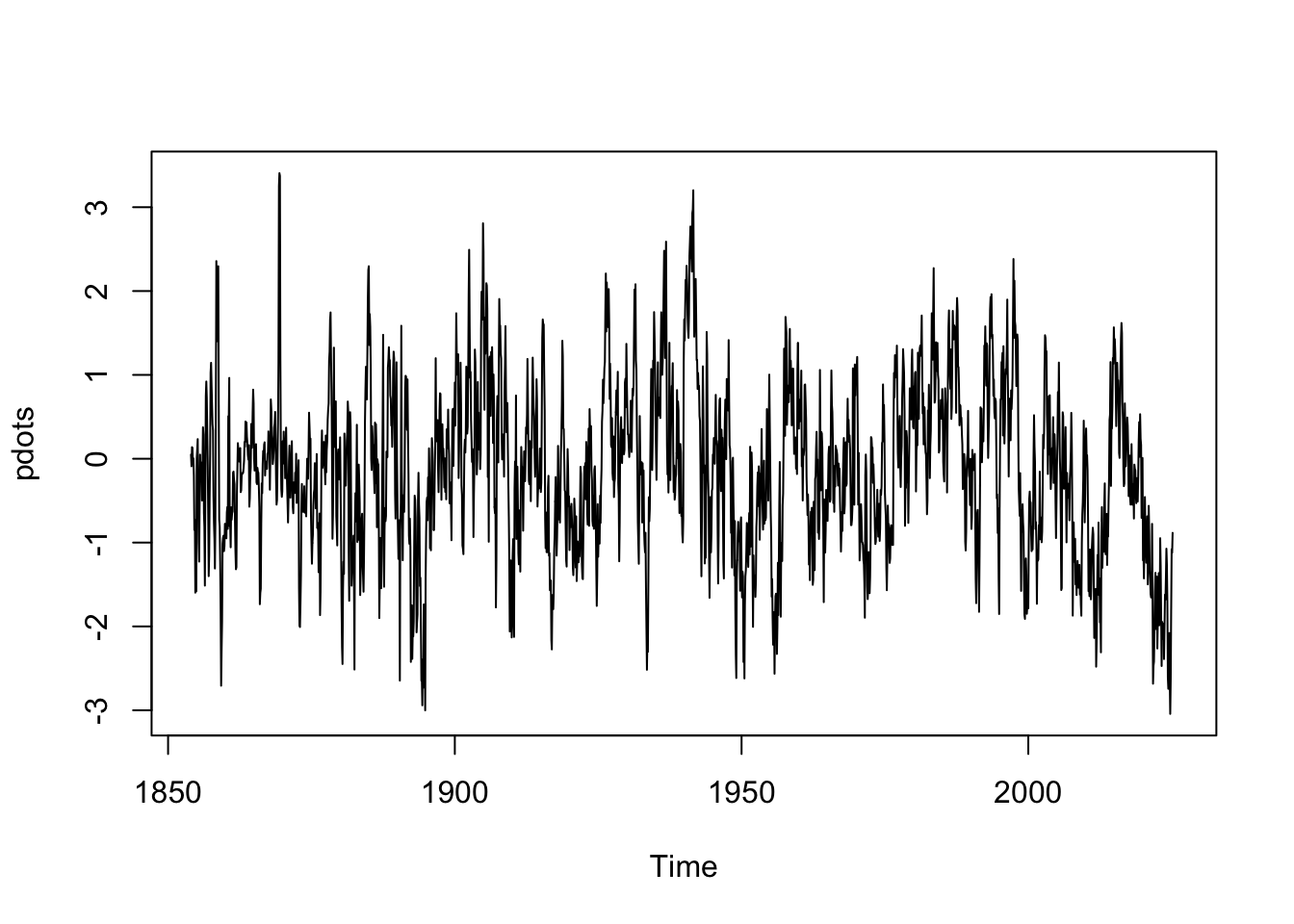

library(atsalibrary)
data("np_climate")
# this has seasonal and annual averages
# use ?np_climate for info
colnames(np_climate_seasonal)

 [1] "year"           "pna.fall"       "pna.spring"     "pna.summer"    
 [5] "pna.winter"     "pna.annual"     "epo.fall"       "epo.spring"    
 [9] "epo.summer"     "epo.winter"     "epo.annual"     "wp.fall"       
[13] "wp.spring"      "wp.summer"      "wp.winter"      "wp.annual"     
[17] "censo.fall"     "censo.spring"   "censo.summer"   "censo.winter"  
[21] "censo.annual"   "whwp.fall"      "whwp.spring"    "whwp.summer"   
[25] "whwp.winter"    "whwp.annual"    "oni.fall"       "oni.spring"    
[29] "oni.summer"     "oni.winter"     "oni.annual"     "meiv2.fall"    
[33] "meiv2.spring"   "meiv2.summer"   "meiv2.winter"   "meiv2.annual"  
[37] "pdo.fall"       "pdo.spring"     "pdo.summer"     "pdo.winter"    
[41] "pdo.annual"     "ipotpi.fall"    "ipotpi.spring"  "ipotpi.summer" 
[45] "ipotpi.winter"  "ipotpi.annual"  "np.fall"        "np.spring"     
[49] "np.summer"      "np.winter"      "np.annual"      "pacwarm.fall"  
[53] "pacwarm.spring" "pacwarm.summer" "pacwarm.winter" "pacwarm.annual"
[57] "gmsst.fall"     "gmsst.spring"   "gmsst.summer"   "gmsst.winter"  
[61] "gmsst.annual"  

Prepping your covariates for MARSS()

You need a matrix:

• Columns = time and number of columns must match your data
• Rows = 1 row for each covariate

Example for PDO

Let’s say we want to use the April-June average PDO. We would construct a matrix with ncols being the years and 1 row for spring PDO.

# col 1 is year
years <- which(np_climate_seasonal$year %in% 2000:2024)
spring_pdo <- np_climate_seasonal$pdo.spring[years]
cmat <- matrix(spring_pdo, nrow=1)
cmat

           [,1]       [,2]   [,3]      [,4]  [,5]      [,6]       [,7]  [,8]
[1,] -0.4936667 -0.8706667 -0.855 0.2236667 0.101 0.6923333 -0.1836667 -0.09
          [,9]     [,10]      [,11]     [,12]  [,13]      [,14]     [,15]
[1,] -1.490333 -1.181667 -0.2626667 -1.055333 -1.271 -0.6396667 0.4516667
         [,16]    [,17] [,18]      [,19] [,20]  [,21] [,22]  [,23]     [,24]
[1,] 0.6253333 1.264333 0.337 -0.5083333  0.22 -0.785 -1.57 -1.748 -2.190333
         [,25]
[1,] -2.347333

This is now \(\mathbf{c}_t\) in \[ \mathbf{x}_t = \mathbf{x}_{t-1} + \mathbf{u} + \mathbf{C}\mathbf{c}_t + \mathbf{w}_t \]

Use PDO to predict steelhead returns

Idea is that pdo (\(p_t\)) is correlated with the fluctuations in log spawner returns (\(x_t\)).

\[ x_t = x_{t-1} + u + (\alpha p_t + w_t) \] But we have 4 steelhead time series for this example. We can write this as: \[ \begin{bmatrix}x_{1,t}\\x_{2,t}\\x_{3,t}\\x_{4,t}\end{bmatrix}= \begin{bmatrix}x_{1,t-1}\\x_{2,t-1}\\x_{3,t-1}\\x_{4,t-1}\end{bmatrix} + \begin{bmatrix}u_1\\u_2\\u_3\\u_4\end{bmatrix}+ \begin{bmatrix}\alpha_1\\\alpha_2\\\alpha_3\\\alpha_4\end{bmatrix} p_t + \begin{bmatrix}w_1\\w_2\\w_3\\w_4\end{bmatrix} \]

What about the \(w_t\)’s? How are they related? Let’s say they are independent with unequal variances (the \(x_t\) are diagonal and unequal). What about our observations? Let’s say each \(y_t\) measures one \(x_t\) with independent and equal error (R is diagonal and equal). Let’s fit this model with MARSS.

Wrangle the raw spawner data to get the \(y_t\) for a MARSS model.

library(tidyverse)
load("Data_Images/esa-salmon.rda")
esu <- unique(esa.salmon$esu_dps)
esunum <- which(esu == "Steelhead (Upper Columbia River DPS)")
esuname <- esu[esunum]

dat <- esa.salmon %>% 
  subset(esu_dps == esuname) %>% # get only this ESU
  mutate(log.spawner = log(value)) %>% # create a column called log.spawner
  dplyr::select(esapopname, spawningyear, log.spawner) %>% # get just the columns that I need
  pivot_wider(names_from = "esapopname", values_from = "log.spawner") %>% 
  column_to_rownames(var = "spawningyear") %>% # make the years rownames
  as.matrix() %>% # turn into a matrix with year down the rows
  t() # make time across the columns
# MARSS complains if I don't do this
dat[is.na(dat)] <- NA
# Clean up rownames
tmp <- rownames(dat)
tmp <- stringr::str_replace(tmp, "Steelhead [(]Upper Columbia River DPS[)]", "")
tmp <- stringr::str_replace(tmp, "River - summer", "")
tmp <- stringr::str_trim(tmp)
rownames(dat) <- tmp

Update your atsalibrary to version 1.6 to get the climate data or load np_climate.RData from the Data_Images directory.

install.packages('atsalibrary', repos = c('https://atsa-es.r-universe.dev', 'https://cloud.r-project.org'))

We will use spring PDO (Apr-Jun).

library(atsalibrary)
data("np_climate")
years <- which(np_climate_seasonal$year %in% colnames(dat))
spring_pdo <- np_climate_seasonal$pdo.spring[years]
cmat <- matrix(spring_pdo, nrow=1)
# No NAs allowed. Interpolate if needed
any(is.na(cmat))

[1] FALSE

Check that cmat and dat have the same number of columns (years).

dim(cmat)

[1]  1 63

dim(dat)

[1]  4 63

Specify a model

# pdo
mod.list1 <- list(
  U = "unequal",
  R = "diagonal and equal",
  Q = "diagonal and unequal",
  c = cmat,
  C = "unequal"
)

# no pdo
mod.list2 <- list(
  U = "unequal",
  R = "diagonal and equal",
  Q = "diagonal and unequal")

library(MARSS)
fit1 <- MARSS(dat, model=mod.list1)

Success! abstol and log-log tests passed at 278 iterations.
Alert: conv.test.slope.tol is 0.5.
Test with smaller values (<0.1) to ensure convergence.

MARSS fit is
Estimation method: kem 
Convergence test: conv.test.slope.tol = 0.5, abstol = 0.001
Estimation converged in 278 iterations. 
Log-likelihood: -153.0968 
AIC: 340.1936   AICc: 344.3569   
 
                            Estimate
R.diag                       0.09599
U.X.Entiat                  -0.00450
U.X.Methow                  -0.00616
U.X.Okanogan                -0.03111
U.X.Wenatchee               -0.01993
Q.(X.Entiat,X.Entiat)        0.12438
Q.(X.Methow,X.Methow)        0.13116
Q.(X.Okanogan,X.Okanogan)    0.11505
Q.(X.Wenatchee,X.Wenatchee)  0.36533
x0.X.Entiat                  5.52606
x0.X.Methow                  7.33549
x0.X.Okanogan                7.45314
x0.X.Wenatchee               8.12444
C.X.Entiat                  -0.07523
C.X.Methow                  -0.02873
C.X.Okanogan                -0.08870
C.X.Wenatchee                0.05881
Initial states (x0) defined at t=0

Standard errors have not been calculated. 
Use MARSSparamCIs to compute CIs and bias estimates.

fit2 <- MARSS(dat, model=mod.list2)

Success! abstol and log-log tests passed at 304 iterations.
Alert: conv.test.slope.tol is 0.5.
Test with smaller values (<0.1) to ensure convergence.

MARSS fit is
Estimation method: kem 
Convergence test: conv.test.slope.tol = 0.5, abstol = 0.001
Estimation converged in 304 iterations. 
Log-likelihood: -154.5953 
AIC: 335.1906   AICc: 337.6012   
 
                            Estimate
R.diag                       0.08492
U.X.Entiat                   0.00213
U.X.Methow                  -0.00557
U.X.Okanogan                -0.00920
U.X.Wenatchee               -0.02427
Q.(X.Entiat,X.Entiat)        0.14095
Q.(X.Methow,X.Methow)        0.14800
Q.(X.Okanogan,X.Okanogan)    0.14483
Q.(X.Wenatchee,X.Wenatchee)  0.38490
x0.X.Entiat                  5.57099
x0.X.Methow                  7.40887
x0.X.Okanogan                7.10616
x0.X.Wenatchee               8.06274
Initial states (x0) defined at t=0

Standard errors have not been calculated. 
Use MARSSparamCIs to compute CIs and bias estimates.

Which one fits better based on AIC? The model without PDO is better (lower AICc).

fit1$AICc

[1] 344.3569

fit2$AICc

[1] 337.6012

Resources

Chapter 7 MARSS models. ATSA Lab Book. https://atsa-es.github.io/atsa-labs/chap-mss.html

Chapter 8 MARSS models with covariates. ATSA Lab Book. https://atsa-es.github.io/atsa-labs/chap-msscov.html

Chapter 16 Modeling cyclic sockeye https://atsa-es.github.io/atsa-labs/chap-cyclic-sockeye.html