2  Lab Intro

Lab 1 Forecasting with ARIMA models

For this lab you will use the material you have learned in the first 3 lectures to explore features of time series of salmon in the North Pacific (Alaska and E Asia). Then you will use ARIMA models to create forecasts and ask a research question with those forecasts.

Teams

1. Bristol Bay Data: Nick Chambers (SAFS), Liz Elmstrom (SAFS), Maria Kuruvilla (QERM)
2. Bristol Bay Data: Eric French (Civil), Dylan Hubl (ESRM), Miranda Mudge (Molecular & Cell Bio)
3. Ruggerone & Irvine Data: Zoe Rand (QERM), Madison Shipley (SAFS), Emma Timmins-Schiffman (Genome Sci)
4. Ruggerone & Irvine Data: Terrance Wang (SAFS), Josh Zahner (SAFS), Karl Veggerby (SAFS)

References

Holmes, E. E. (2020) Fisheries Catch Forecasting https://fish-forecast.github.io/Fish-Forecast-Bookdown

Hyndman, R.J., & Athanasopoulos, G. (2018) Forecasting: principles and practice, 2nd edition, OTexts: Melbourne, Australia. https://otexts.com/fpp2/.

Plus the lecture material on the ATSA website.

Type of questions you might ask

“Compare the accuracy of forecasts using best fit ARIMA models for pink salmon using the different regions in the Ruggerone & Irvine data. Is forecast accuracy is different for different regions?”

“Compare the accuracy of total abundance forecasts using ARIMA models for Bristol Bay sockeye rivers and compare to the AKFW and UW FRI forecasts.”

“Compare the accuracy of age-group forecasts using ARIMA models for Bristol Bay sockeye and compare to the AKFW and UW FRI forecasts.”

“Use the Ruggerone & Irvine data and ARIMA models to study the autoregressive structure of pink, chum and sockeye. Are there differences by region (AK verus E Asia)?”

“Compare the forecasts of total North Pacific pink and chum using 5, 10, 15, and 20 years of training data. Does forecast accuracy increase with more training data?”

“Create 1-year forecasts of total North Pacific pink salmon using 20 years of training data for all of the Ruggerone and Irvine data. Is forecast error correlated with the PDO?”

Bristol Bay Sockeye data

The bristol_bay_data_plus_covariates.rds file has Bristol Bay sockeye abundance for 9 rivers for 4 age-groups. The data are from Ovando et al 2021 Improving forecasts of sockeye salmon (Oncorhynchus nerka) with parametric and nonparametric models DOI: 10.1139/cjfas-2021-0287. You’ll find a copy in the lab folder. The data file also has the covariates for year that the smolts enter the ocean as used in Ovando et al. 

Load the data.

Code

bb_data <- readRDS(here::here("Lab-1", "Data_Images", "bristol_bay_data_plus_covariates.rds"))

The data you will most likely want are

• ret_yr The year the spawners return to the spawning grounds
• ret The returns (number of fish in 1000s)
• system The river name
• age_group The age_group
• forecast.adfw The forecast from AK Fish and Wildlife
• forecast.fri The forecast from UW Fisheries Research Institute
• env_* are some covariates at the year the age group entered the ocean

In the data file, the age group designation is “a.b” where “a” is number of years in freshwater and “b” is number of years in the ocean. The age of the spawners in then a+b.

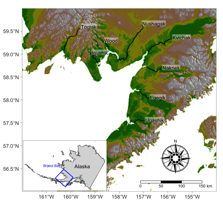
The data

colnames:  brood_yr ret_yr system fw_age o_age age_group ret forecast.adfw forecast.fri env_pdo env_sst env_slp env_upstr 

system (river):  Igushik Wood Nushagak Kvichak Naknek Egegik Ugashik 

age groups:  

Some plots of the Bristol Bay data. Hmm there is a NA that was replaced with 0 it looks like.

Code

bb_data %>% 
  filter(system=="Kvichak") %>% 
  ggplot(aes(x=ret_yr, y=log(ret))) + 
    geom_line() + 
    ggtitle("log abundance by age group") +
    facet_wrap(~age_group)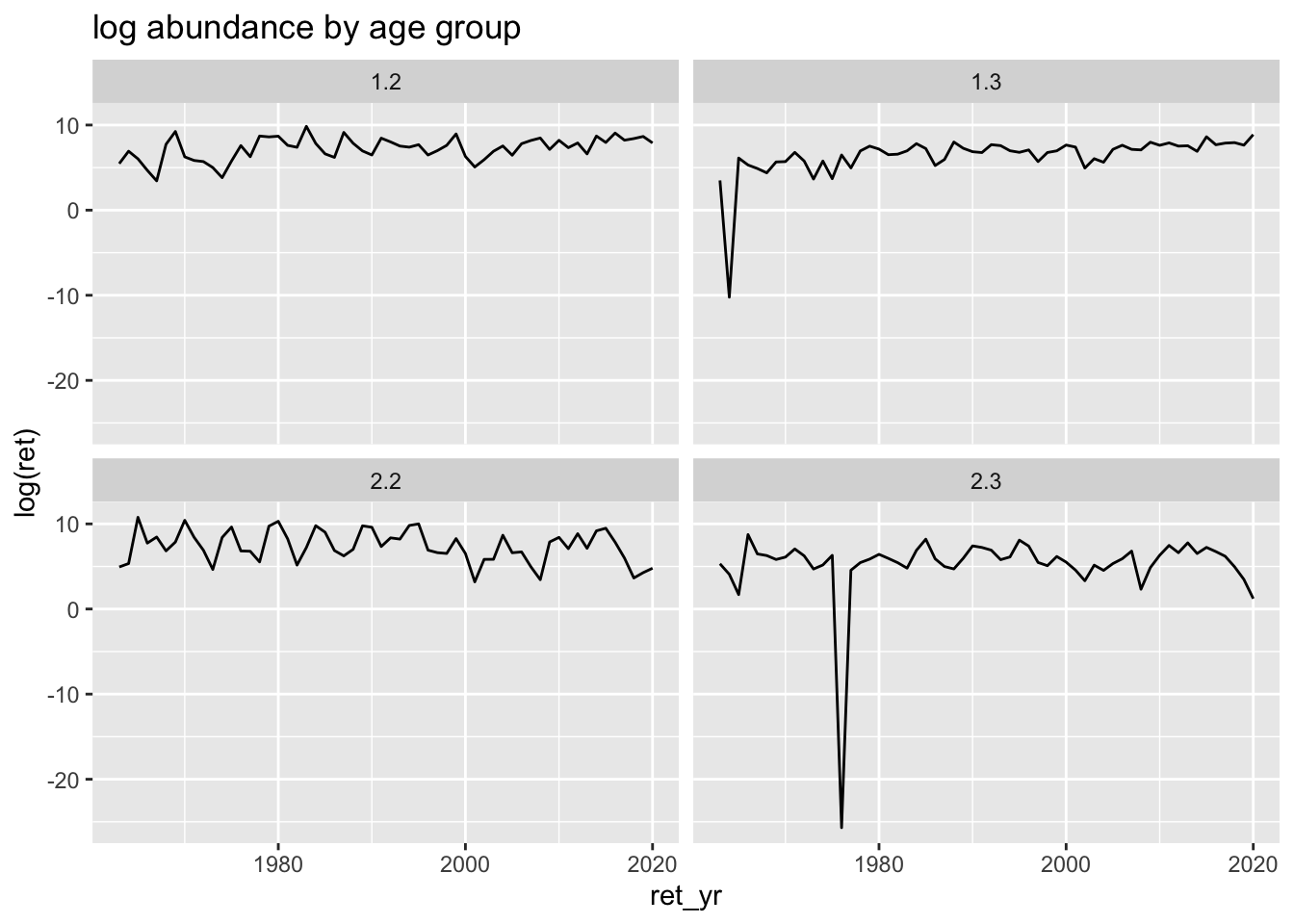

plotted by age group

Code

bb_data %>% 
  group_by(system, ret_yr) %>%
  summarize(total = sum(ret, na.rm=TRUE)) %>%
  ggplot(aes(x=ret_yr, y=log(total))) + 
    geom_line() + 
    ggtitle("log abundance by river") +
    facet_wrap(~system)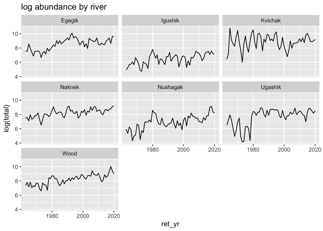

total across all 4 ages

Some subsets of the data

Here are some subsets of the data that you might want to use.

Log total by age group

Code

subdata <- bb_data %>% 
  group_by(age_group, ret_yr) %>%
  summarize(lntotal = log(sum(ret, na.rm=TRUE)))
head(subdata)

# A tibble: 6 × 3
# Groups:   age_group [1]
  age_group ret_yr lntotal
  <chr>      <dbl>   <dbl>
1 1.2         1963    7.49
2 1.2         1964    8.50
3 1.2         1965    7.22
4 1.2         1966    7.18
5 1.2         1967    6.88
6 1.2         1968    8.11

Log total by river

Code

subdata <- bb_data %>% 
  group_by(system, ret_yr) %>%
  summarize(lntotal = log(sum(ret, na.rm=TRUE)))
head(subdata)

# A tibble: 6 × 3
# Groups:   system [1]
  system ret_yr lntotal
  <chr>   <dbl>   <dbl>
1 Egegik   1963    7.54
2 Egegik   1964    7.55
3 Egegik   1965    8.55
4 Egegik   1966    7.95
5 Egegik   1967    7.41
6 Egegik   1968    6.88

Compare fish that spend 2 years in ocean versus those that spend 3 years.

Code

subdata <- bb_data %>% 
  mutate(
    ocean_years = case_match(
      age_group, 
      c("2.3", "1.3") ~ "3-yr-ocean",
      c("1.2", "2.2") ~ "2-yr-ocean",
      .default = age_group
    )) %>%
  group_by(system, ocean_years, ret_yr) %>%
  summarize(lntotal = log(sum(ret, na.rm=TRUE)))
head(subdata)

# A tibble: 6 × 4
# Groups:   system, ocean_years [1]
  system ocean_years ret_yr lntotal
  <chr>  <chr>        <dbl>   <dbl>
1 Egegik 2-yr-ocean    1963    7.02
2 Egegik 2-yr-ocean    1964    7.29
3 Egegik 2-yr-ocean    1965    8.34
4 Egegik 2-yr-ocean    1966    5.96
5 Egegik 2-yr-ocean    1967    6.58
6 Egegik 2-yr-ocean    1968    6.35

Get one time series and split into train and test. Each with 10 years.

Code

dat <- bb_data %>%
  filter(system == "Kvichak", age_group == "1.3") %>%
  mutate(lnreturns = log(ret),
         year = ret_yr) %>%
  select(year, lnreturns)
datts <- ts(dat$lnreturns, start=dat$year[1])
train <- window(datts, dat$year[1], dat$year[1]+9)
test <- window(datts, dat$year[1]+10, dat$year[1]+10+9)

Ruggerone & Irvine: Salmon in the North Pacific

The data set Data_Images/ruggerone_data.rds has total abundance of natural spawners (not hatchery) from 15 regions in the N Pacific. These are data provided with Ruggerone, G. and Irvine, J. 2018. Numbers and biomass of natural- and hatchery-origin Pink, Chum, and Sockeye Salmon in the North Pacific Ocean, 1925-2015. Marine and Coastal Fisheries: Dynamics, Management, and Ecosystem Science 10. DOI: 10.1002/mcf2.10023. Open Access.

Load the data

Code

ruggerone_data <- readRDS(here::here("Lab-1", "Data_Images", "ruggerone_data.rds"))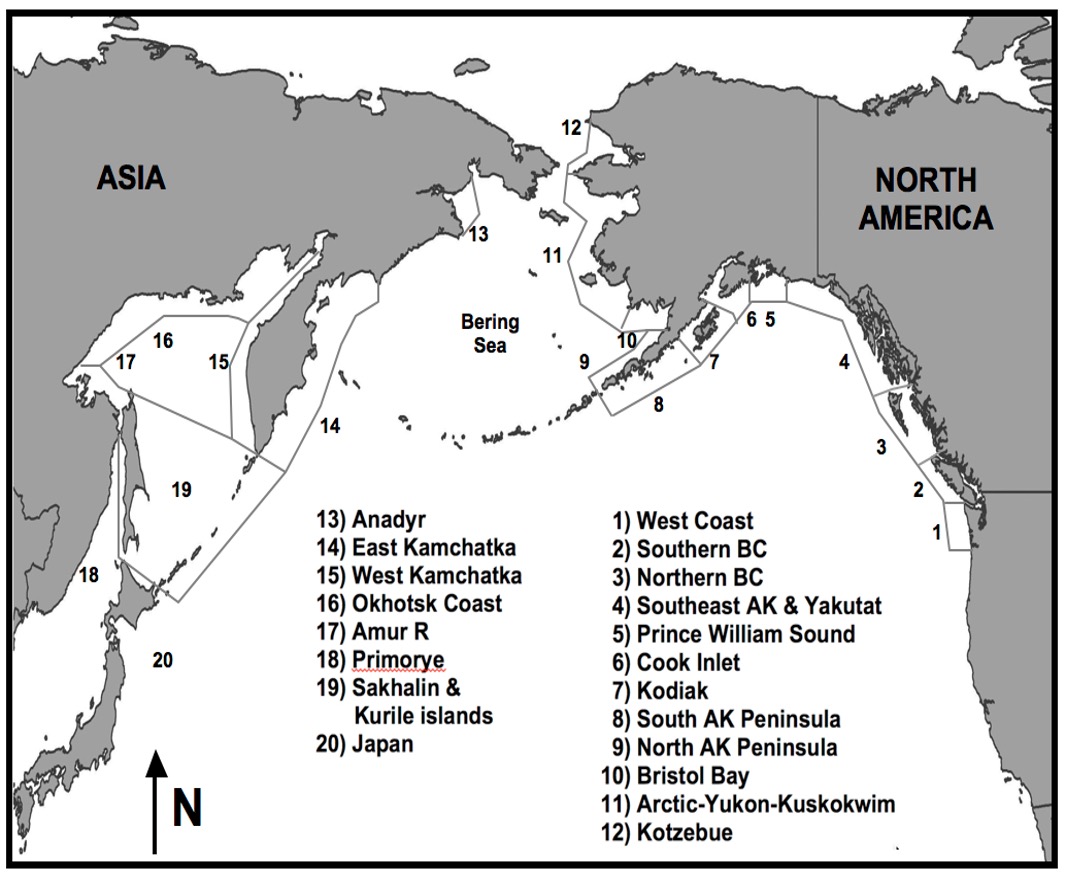

Figure 1. The approximate geographic locations of regional stock groups. Region 1, Washington State, including the Columbia River. Region 2, Southern British Columbia (BC) south of the central coast of British Columbia (~51°N). . Region 3, Northern BC including central and northern British Columbia. Region 4, Southeast Alaska (AK) including the Yakutat coast. The Central Alaska region extends from the Bering River (~60°N), near Prince William Sound in Region 5, westward to Unimak Island (~166°W), thereby including Regions 5 through 8. Western Alaska includes Regions 9 through 12, i.e., all North American drainages flowing into the Bering Sea from Unimak Island to Kotzebue. Data for eastern and western Kamchatka (Regions 14 and 15) are separated from data for the Russian mainland and islands (called “Mainland & Islands” here, which includes the Okhotsk coast, Amur River, Primorye, Sakhalin and Kurile Islands, and relatively small runs to the Anadyr). Region 20, Japan, includes the islands of Hokkaido and Honshu. South Korea (Region 21) not shown.

region in data file	desciption	regions in map
japan	Japan & South Korea	20 and 21
m_i	Russian Mainland & Islands	13, 16, 17 18, 19
w_kam	Western Kamchatka	15
e_kam	Eastern Kamchatka	14
wak	Western Alaska	9, 10, 11, 12
s_pen	Southern Alaska Peninsula	8
kod	Kodiak	7
ci	Cook Inlet	6
pws	Prince William Sound	5
seak	Southeast Alaska	4
nbc	Northern British Columbia	3
sbc	Southern British Columbia	2
wa	Washington State	1
wc	West Coast USA	mislabeled on map
cak (not in data file)	Central Alaska	5, 6, 7, 8

Ruggerone and Irvine data

colnames:  year region returns species 

species:  pink chum sockeye 

regions:  ci e_kam japan kod korea m_i nbc pws sbc seak s_pen wa wak w_kam wc 

Some plots of the Ruggerone and Irvine data.

Code

ruggerone_data %>% 
  filter(species=="pink") %>% 
  ggplot(aes(x=year, y=log(returns))) + 
    geom_line() + 
    ggtitle("pink salmon log abundance") +
    facet_wrap(~region)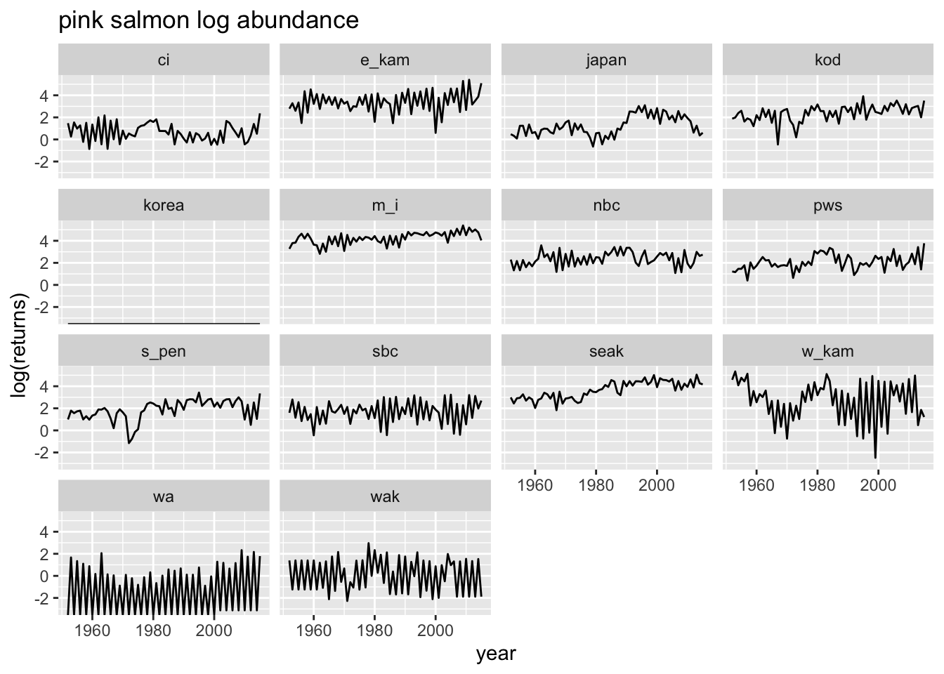

pink salmon by regions

Code

ruggerone_data %>% 
  group_by(species, year) %>%
  summarize(total = sum(returns, na.rm=TRUE)) %>%
  ggplot(aes(x=year, y=log(total))) + 
    geom_line() + 
    ggtitle("log abundance by species") +
    facet_wrap(~species)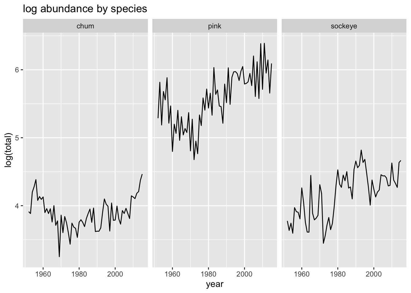

total by species

Some subsets of the data

Here are some subsets of the data that you might want to use.

Log total North Pacific pink, chum, sockeye

Code

subdata <- ruggerone_data %>% 
  group_by(species, year) %>%
  summarize(lntotal = log(sum(returns, na.rm=TRUE)))
head(subdata)

# A tibble: 6 × 3
# Groups:   species [1]
  species  year lntotal
  <chr>   <dbl>   <dbl>
1 chum     1952    3.91
2 chum     1953    3.88
3 chum     1954    4.20
4 chum     1955    4.28
5 chum     1956    4.38
6 chum     1957    4.08

Log North Pacific pink

Code

subdata <- ruggerone_data %>% 
  filter(species == "pink") %>%
 mutate(lnreturns = log(returns))
head(subdata)

# A tibble: 6 × 5
   year region returns species lnreturns
  <dbl> <chr>    <dbl> <chr>       <dbl>
1  1952 ci       4.36  pink        1.47 
2  1953 ci       1.30  pink        0.264
3  1954 ci       4.67  pink        1.54 
4  1955 ci       2.67  pink        0.981
5  1956 ci       3.57  pink        1.27 
6  1957 ci       0.804 pink       -0.218

Total in some bigger areas

Code

subdata <- ruggerone_data %>% 
  mutate(
    area = case_match(
      region, 
      c("japan", "korea", "m_i", "e_kam", "w_kam") ~ "East_Asia",
      c("wak", "s_pen", "kod", "ci", "pws", "seak") ~ "Alaska",
      c("nbc", "sbc", "wa", "wc") ~ "WC",
      .default = region
    )) %>%
  group_by(area, species, year) %>%
  summarize(lntotal = log(sum(returns, na.rm=TRUE)))
head(subdata)

# A tibble: 6 × 4
# Groups:   area, species [1]
  area   species  year lntotal
  <chr>  <chr>   <dbl>   <dbl>
1 Alaska chum     1952    2.83
2 Alaska chum     1953    2.77
3 Alaska chum     1954    2.92
4 Alaska chum     1955    2.47
5 Alaska chum     1956    2.81
6 Alaska chum     1957    2.89

Example analysis

Get one time series out of ruggerone_data

Code

dat <- ruggerone_data %>%
  filter(region == "wak", species == "pink") %>%
  mutate(lnreturns = log(returns)) %>%
  select(year, lnreturns)
head(dat)

# A tibble: 6 × 2
   year lnreturns
  <dbl>     <dbl>
1  1952      1.40
2  1953     -1.24
3  1954      1.40
4  1955     -1.24
5  1956      1.40
6  1957     -1.24

Make a time series object and divide into train and test data.

Code

datts <- ts(dat$lnreturns, start=dat$year[1])
train <- window(datts, 1952, 1971)
test <- window(datts, 1972, 2001)

Fit a model with auto.arima() in the forecast package.

Code

library(forecast)
mod <- auto.arima(train)
mod

Series: train 
ARIMA(1,0,0) with zero mean 

Coefficients:
          ar1
      -0.9293
s.e.   0.0725

sigma^2 = 0.3815:  log likelihood = -19.22
AIC=42.45   AICc=43.15   BIC=44.44

Plot a 30-year forecast against the test data.

Code

library(zoo)

Attaching package: 'zoo'

The following objects are masked from 'package:base':

    as.Date, as.Date.numeric

Code

fr <- forecast(mod, h=30)
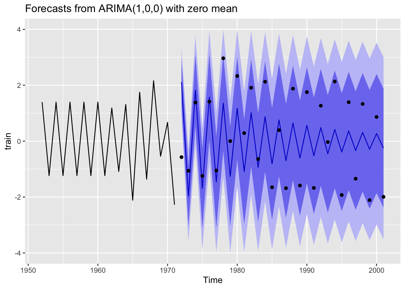
autoplot(fr) + geom_point(aes(x=x, y=y), data=fortify(test))