dfaTMB: Dynamic Factor Analysis

dfaTMB() will be replaced with MARSS(..., method="TMB")

The dfaTMB() function allows you to fit DFAs with the same form as MARSS(x, form="dfa"). This has a diagonal \(\mathbf{Q}\) with 1 on the diagonal and a stochastic \(\mathbf{x}_1\) with mean 0 and variance of 5 (diagonal variance-covariance matrix). There are only 3 options allowed for \(\mathbf{R}\): diagonal and equal, diagonal and unequal, and unconstrained.

Example data

library(MARSS)
data(lakeWAplankton, package = "MARSS")
phytoplankton <- c("Cryptomonas", "Diatoms", "Greens", "Unicells", "Other.algae")
dat <- as.data.frame(lakeWAplanktonTrans) |>
  subset(Year >= 1980 & Year <= 1989) |>
  subset(select=phytoplankton) |>
  t() |>
  MARSS::zscore()

Fit with MARSS

m1.em <- MARSS(dat, model=list(R='unconstrained', m=1, tinitx=1), form='dfa', z.score=FALSE, silent = TRUE)

Fit with TMB. Note the syntax will be updated to match MARSS().

library(marssTMB)
m1.tmb <- dfaTMB(dat, model=list(m=1, R='unconstrained'))

Compare parameter estimates

library(tidyr)
pars <- data.frame(name = c(paste0("R", rownames(coefficients(m1.em)$R)),
                            paste0("Z", rownames(coefficients(m1.em)$Z))),
                   EM = c(coefficients(m1.em)$R, coefficients(m1.em)$Z),
  TMB = c(as.vector(m1.tmb$Estimates$R[lower.tri(m1.tmb$Estimates$R,diag=TRUE)]),
  as.vector(m1.tmb$Estimates$Z)))
pars <- pars %>% tidyr::pivot_longer(2:3, names_to = "model")

library(ggplot2)
dodge <- position_dodge(width=0.5)
ggplot(pars, aes(x=name, y=value, col=model)) +
  geom_point(position=dodge) +
  ggtitle("same estimates")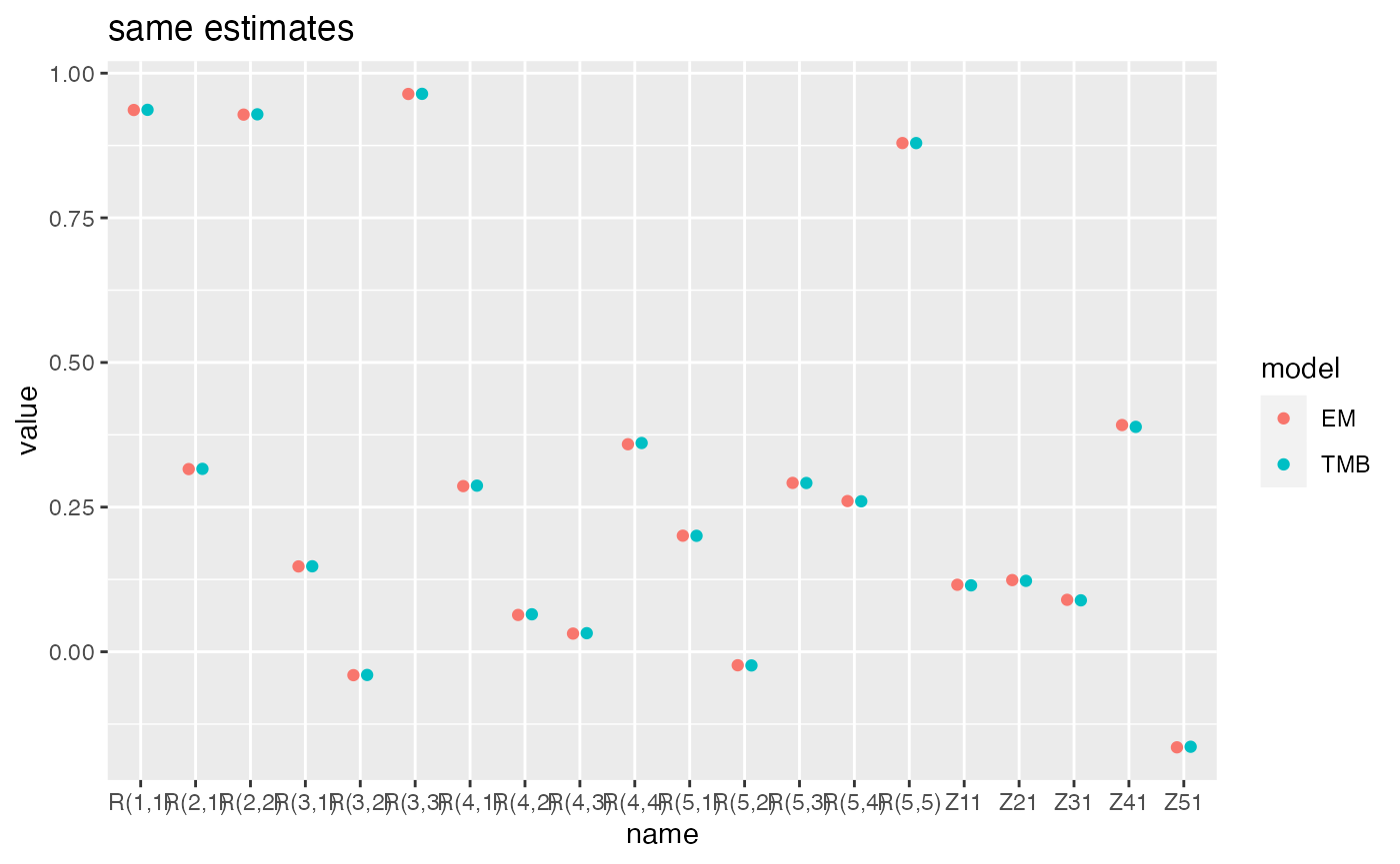

Compare two states models.

m1.bfgs <- MARSS(dat, model=list(R='unconstrained', m=2, tinitx=1), form='dfa', z.score=FALSE, silent = TRUE,
               method="BFGS")
m1.tmb <- dfaTMB(dat, model=list(m=2, R='unconstrained'))
c(m1.bfgs$logLik, m1.tmb$logLik)
#> [1] -765.8454 -765.8454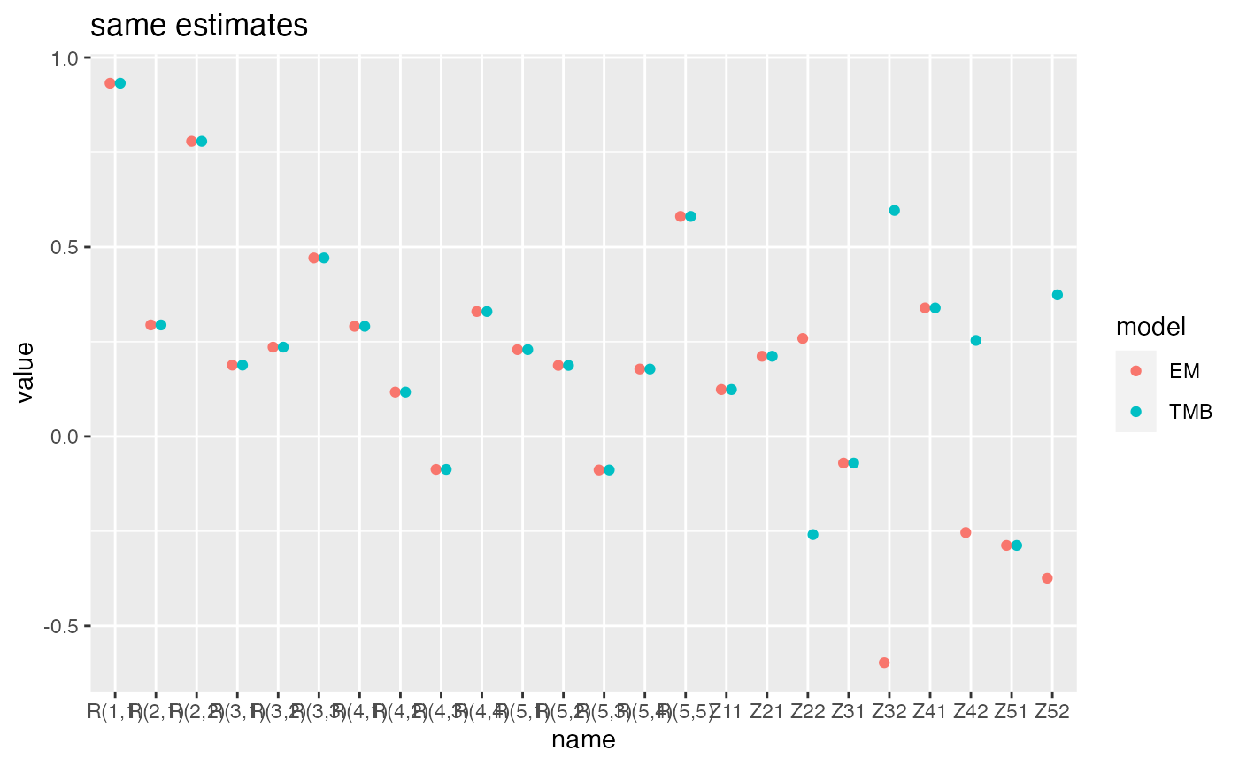

Compare two states models with R diagonal and equal

mod.list <- list(R='diagonal and equal', m=2, tinitx=1)
m1.bfgs <- MARSS(dat, model=mod.list, form='dfa', z.score=FALSE, silent = TRUE,
               method="BFGS")
m1.tmb <- dfaTMB(dat, model=mod.list)
c(m1.bfgs$logLik, m1.tmb$logLik)
#> [1] -798.3209 -798.3209

Include a comparison with covariates

data(lakeWAplankton, package = "MARSS")
phytoplankton <- c("Cryptomonas", "Diatoms", "Greens", "Unicells", "Other.algae")
dat <- as.data.frame(lakeWAplanktonTrans) |>
  subset(Year >= 1980 & Year <= 1989) |>
  subset(select=phytoplankton) |>
  t() |>
  MARSS::zscore()

# add a temperature covariate
temp <- as.data.frame(lakeWAplanktonTrans) |>
    subset(Year >= 1980 & Year <= 1989) |>
    subset(select=Temp)
covar <- t(temp)
m_cov_tmb <- dfaTMB(dat, model=list(m=1, R='diagonal and unequal'), 
                    EstCovar = TRUE, Covars = covar)
m_cov_tmb$Estimates$D
#>             [,1]
#> [1,]  0.05906647
#> [2,] -0.27764610
#> [3,]  0.50726835
#> [4,]  0.13172004
#> [5,]  0.53792693

# add a 2nd covariate
TP <- as.data.frame(lakeWAplanktonTrans) |>
    subset(Year >= 1980 & Year <= 1989) |>
    subset(select=TP)
covar <- rbind(covar, t(TP))
m_cov2_tmb <- dfaTMB(dat, model=list(m=1, R='diagonal and unequal'), 
                    EstCovar = TRUE, Covars = covar)
m_cov2_tmb$Estimates$D
#>             [,1]        [,2]
#> [1,]  0.01241099 -0.27750487
#> [2,] -0.32294643 -0.26915892
#> [3,]  0.49174949 -0.09746135
#> [4,]  0.10052332 -0.19418803
#> [5,]  0.53275591 -0.02629113

Look at a bigger data set

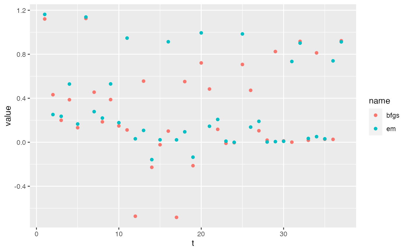
Compare three states models with R diagonal and unequal and 12 time series. The EM algorithm and TMB algorithms struggles to converge with DFA models. This is specific to this set of time series.

dat2 <- rbind(dat, dat+matrix(rnorm(nrow(dat)*ncol(dat),0,0.2), nrow(dat), ncol(dat)))
dat2 <- MARSS::zscore(dat2)
mod.list <- list(R='diagonal and unequal', m=3, tinitx=1)
# Control set to match setting in MARSS.tmp()
t1.bfgs <- system.time(m1.bfgs <- MARSS(dat2, 
                                        model=mod.list, form='dfa', 
                                        z.score=FALSE, silent = TRUE, method="BFGS", 
                                        control = list(reltol = 1e-12, maxit=2000)))[1]
t1.em <- system.time(m1.em <- MARSS(dat2, model=mod.list, form='dfa', z.score=FALSE, silent = TRUE))[1]
t1.tmb <- system.time(m1.tmb <- dfaTMB(dat2, model=mod.list))[1]
t1.tmb2 <- system.time(m1.tmb2 <- dfaTMB(dat2, model=mod.list, fun.opt="optim"))[1]

TMB + nlminb() is much faster. But at the default convergence settings, the Kalman-Filter + BFGS ran longer and got to a higher maximum likelihood. This seems to be an issue with TMB for both the optimizers. Also the speed savings seems to be due to nlminb() not TMB per se.

# Log-likelihood
c(em=m1.em$logLik, kfoptim=m1.bfgs$logLik, TMBnlminb=m1.tmb$logLik, TMBoptim=m1.tmb2$logLik)
#>        em   kfoptim TMBnlminb  TMBoptim 
#> -1096.381 -1036.093 -1096.186 -1269.752
# Time
c(em=t1.em, kfoptim=t1.bfgs, TMBnlminb=t1.tmb, TMBoptim=t1.tmb2)
#>        em.user.self   kfoptim.user.self TMBnlminb.user.self  TMBoptim.user.self 
#>               7.185              19.816               1.616               6.253

It might be an odd initial condition issue as if BFGS is started with EM, it does not find the lower log-likelihood but ends up at the higher value that EM and TMB found. Note, this varies a bit. This is for set.seed(1234).

m1 <- MARSS(dat2, model=mod.list, form='dfa', z.score=FALSE, silent = TRUE, control = list(minit=1, maxit=10))

t2.bfgs <- system.time(m2.bfgs <- MARSS(dat2, model=mod.list, form='dfa', z.score=FALSE, silent = TRUE, method="BFGS", inits = m1))[1]
c(t2.bfgs, m2.bfgs$logLik)
#> user.self           
#>     4.317 -1096.186

df <- data.frame(t=1:37, bfgs=tidy(m1.bfgs)$estimate, em=tidy(m1.em)$estimate) |>
  pivot_longer(2:3)
ggplot(df, aes(x=t, y=value, col=name)) + geom_point()

Eli Holmes

2023-05-15

Include a comparison with covariates

Look at a bigger data set