Plot MARSS marssResiduals objects — plot.marssResiduals • MARSS

Plots residuals using the output from a residuals() call. By default all available residuals plots are plotted. Individual plots can be plotted by passing in plot.type. If an individual plot is made using autoplot(), the ggplot object is returned which can be further manipulated. Plots are only shown for those residual types in the marssResiduals object.

Usage

# S3 method for marssResiduals
plot(x, plot.type = c("all", "residuals", "qqplot", "acf"), 
                   conf.int = TRUE, conf.level = 0.95, decorate = TRUE,
                   plot.par = list(), silent = FALSE, ...)
# S3 method for marssResiduals
autoplot(x, 
           plot.type = c("all", "residuals", "qqplot", "acf"), 
           conf.int = TRUE, conf.level = 0.95, decorate = TRUE, 
           plot.par = list(), 
           silent = FALSE)

Arguments

x: A marssResiduals object.
plot.type: Type of plot. If not passed in, all plots are drawn. See details for plot types.
conf.int: TRUE/FALSE. Whether to include a confidence interval.
conf.level: Confidence level for CIs.
decorate: TRUE/FALSE. Add smoothing lines to residuals plots or qqline to qqplots and add data points plus residuals confidence intervals to states and observations plots.
plot.par: A list of plot parameters to adjust the look of the plots. The default is list(point.pch = 19, point.col = "blue", point.fill = "blue", point.size = 1, line.col = "black", line.size = 1, line.linetype = "solid", ci.fill = "grey70", ci.col = "grey70", ci.linetype = "solid", ci.linesize = 0, ci.alpha = 0.6).
silent: No console interaction or output.
...: Not used.

Value

If an individual plot is selected using plot.type and autoplot() is called, then the ggplot object is returned invisibly.

Details

If resids <- residuals(x) is used (default) where x is a marssMLE object from a MARSS() call, then resids has the innovations residuals, or one-step-ahead residuals. These are what are commonly used for residuals diagnostics in state-space modeling. However, other types of residuals are possible for state-space models; see MARSSresiduals() for details. The plot function for marssResiduals objects will handle all types of residuals that might be in the marssResiduals object. However if you simply use the default behavior, resids <- residuals(x) and plot(resids), you will get the standard model residuals diagnostics plots for state-space models, i.e. only model residuals plots and only plots for innovations model residuals (no smoothations model residuals).

The plot types are as follows:

"all": All the residuals in the residuals object plus QQ plots and ACF plots.
"residuals": Only residuals versus time.
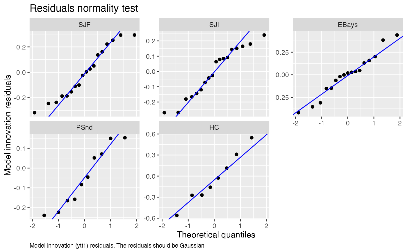
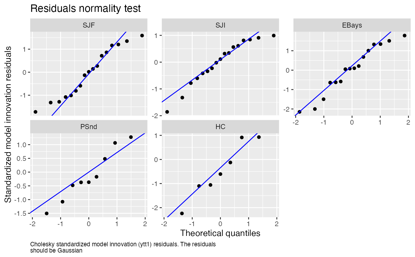
"qqplot": Only QQ plots. Visual normality test for the residuals.
"acf": ACF of the residuals. If x$type is "ytt1", these are the one-step-ahead (aka innovations) residuals and they should be temporally independent.

Author

Eli Holmes

Examples

data(harborSealWA)
model.list <- list( Z = as.factor(c(1, 1, 1, 1, 2)), R = "diagonal and equal")
fit <- MARSS(t(harborSealWA[, -1]), model = model.list)
#> Success! abstol and log-log tests passed at 20 iterations.
#> Alert: conv.test.slope.tol is 0.5.
#> Test with smaller values (<0.1) to ensure convergence.
#> 
#> MARSS fit is
#> Estimation method: kem 
#> Convergence test: conv.test.slope.tol = 0.5, abstol = 0.001
#> Estimation converged in 20 iterations. 
#> Log-likelihood: 18.89262 
#> AIC: -17.78524   AICc: -14.11857   
#>  
#>         Estimate
#> A.SJI    0.79679
#> A.EBays  0.27580
#> A.PSnd  -0.55342
#> R.diag   0.02269
#> U.1      0.05889
#> U.2     -0.00466
#> Q.(1,1)  0.00753
#> Q.(2,2)  0.02486
#> x0.1     6.16171
#> x0.2     6.62763
#> Initial states (x0) defined at t=0
#> 
#> Standard errors have not been calculated. 
#> Use MARSSparamCIs to compute CIs and bias estimates.
#> 
resids <- residuals(fit)

require(ggplot2)
# plots of residuals versus time, QQ-norm plot, and ACF
autoplot(resids)

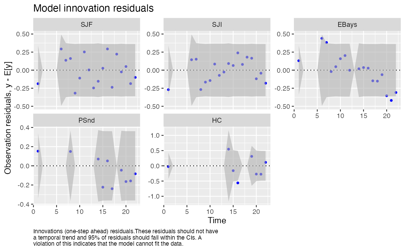#> plot.type = model.resids.ytt1 

#> Hit <Return> to see next plot (q to exit): 

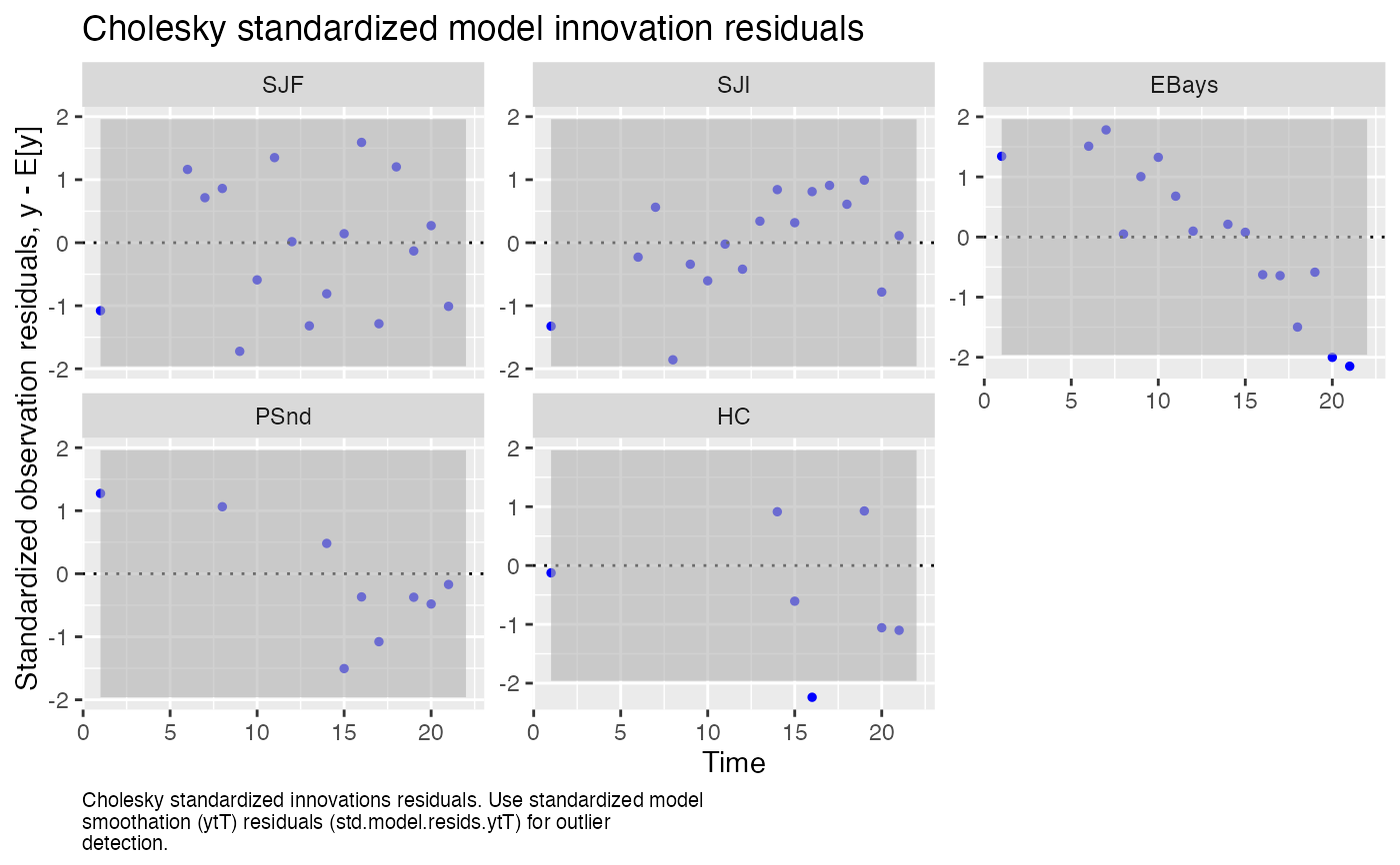#> plot.type = std.model.resids.ytt1 

#> Hit <Return> to see next plot (q to exit): 

#> plot.type = qqplot.model.resids.ytt1 

#> Hit <Return> to see next plot (q to exit): 

#> plot.type = qqplot.std.model.resids.ytt1 

#> Hit <Return> to see next plot (q to exit): 

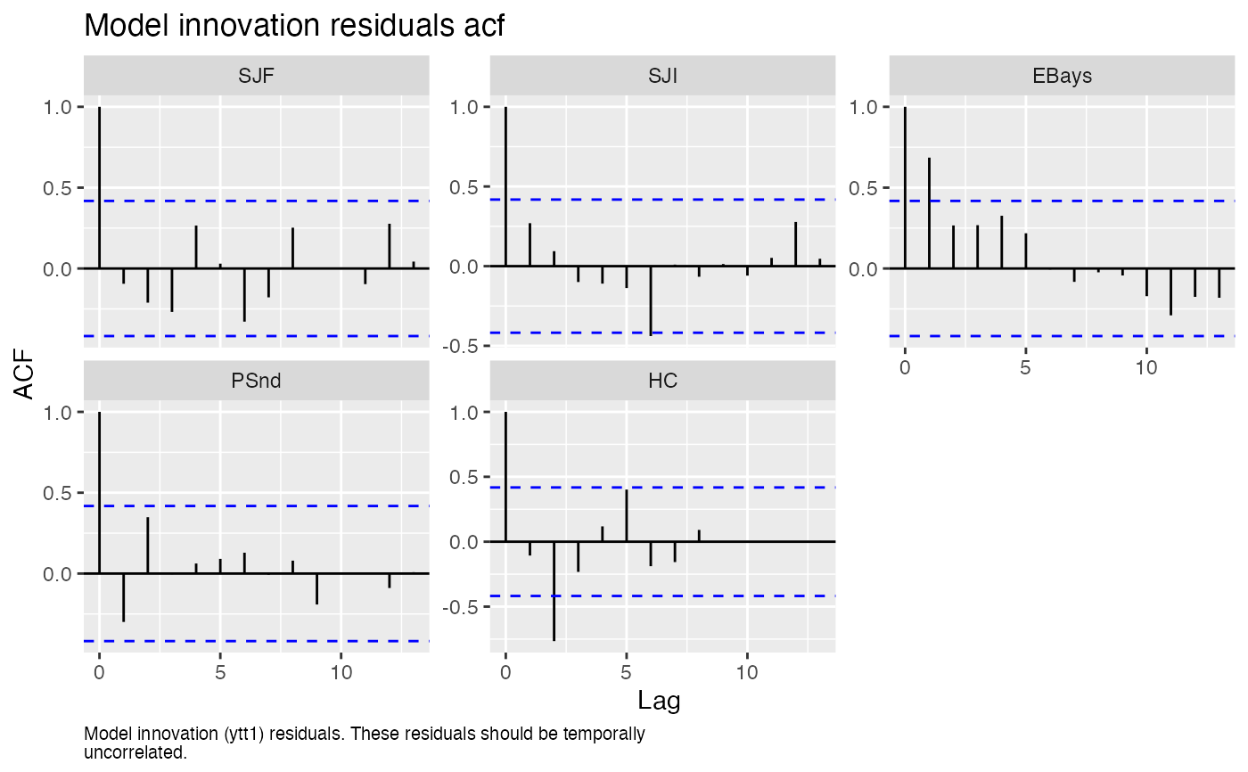#> plot.type = acf.model.resids.ytt1 

#> Hit <Return> to see next plot (q to exit): 

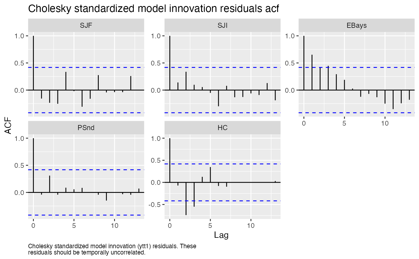#> plot.type = acf.std.model.resids.ytt1 

#> Finished plots.

# only the ACF plots
# autoplot(resids, plot.type = "acf")