Plot MARSS Forecast and Predict objects

Plots forecasts with prediction (default) or confidence intervals using base R graphics (plot) and ggplot2 (autoplot). The plot function is built to mimic plot.forecast in the forecast package in terms of arguments and look.

Usage

# S3 method for marssPredict
plot(x, include, decorate = TRUE, main = NULL, showgap = TRUE, 
    shaded = TRUE, shadebars = (x$h < 5 & x$h != 0), shadecols = NULL, col = 1, 
    fcol = 4, pi.col = 1, pi.lty = 2, ylim = NULL, 
    xlab = "", ylab = "", type = "l", flty = 1, flwd = 2, ...)
# S3 method for marssPredict
autoplot(x, include, decorate = TRUE, plot.par = list(),  ...)

Arguments

x

marssPredict produced by forecast.marssMLE() or predict.marssMLE().

include

number of time step from the training data to include before the forecast. Default is all values.

main

Text to add to plot titles.

showgap

If showgap=FALSE, the gap between the training data and the forecasts is removed.

shaded

Whether prediction intervals should be shaded (TRUE) or lines (FALSE).

shadebars

Whether prediction intervals should be plotted as shaded bars (if TRUE) or a shaded polygon (if FALSE). Ignored if shaded=FALSE. Bars are plotted by default if there are fewer than five forecast horizons.

shadecols

Colors for shaded prediction intervals.

col

Color for the data line.

fcol

Color for the forecast line.

pi.col

If shaded=FALSE and PI=TRUE, the prediction intervals are plotted in this color.

pi.lty

If shaded=FALSE and PI=TRUE, the prediction intervals are plotted using this line type.

ylim

Limits on y-axis.

xlab

X-axis label.

ylab

Y-axis label.

type

Type of plot desired. As for plot.default.

flty

Line type for the forecast line.

flwd

Line width for the forecast line.

...

Other arguments, not used.

decorate

TRUE/FALSE. Add data points and CIs or PIs to the plots.

plot.par

A list of plot parameters to adjust the look of the plot. The default is list(point.pch = 19, point.col = "blue", point.fill = "blue", point.size = 1, line.col = "black", line.size = 1, line.type = "solid", ci.fill = NULL, ci.col = NULL, ci.linetype = "blank", ci.linesize = 0, ci.alpha = 0.6, f.col = "#0000AA", f.linetype = "solid", f.linesize=0.5, theme = theme_bw()).

Value

None. Plots are plotted

Author

Eli Holmes and based off of plot.forecast in the forecast package written by Rob J Hyndman & Mitchell O'Hara-Wild.

See also

predict.marssMLE()

Examples

data(harborSealWA)
dat <- t(harborSealWA[, -1])
fit <- MARSS(dat[1:2,])
#> Success! abstol and log-log tests passed at 17 iterations.
#> Alert: conv.test.slope.tol is 0.5.
#> Test with smaller values (<0.1) to ensure convergence.
#> 
#> MARSS fit is
#> Estimation method: kem 
#> Convergence test: conv.test.slope.tol = 0.5, abstol = 0.001
#> Estimation converged in 17 iterations. 
#> Log-likelihood: 7.867711 
#> AIC: -1.735423   AICc: 2.264577   
#>  
#>                 Estimate
#> R.diag           0.01348
#> U.X.SJF          0.06852
#> U.X.SJI          0.07242
#> Q.(X.SJF,X.SJF)  0.02037
#> Q.(X.SJI,X.SJI)  0.00961
#> x0.X.SJF         6.01228
#> x0.X.SJI         6.74861
#> Initial states (x0) defined at t=0
#> 
#> Standard errors have not been calculated. 
#> Use MARSSparamCIs to compute CIs and bias estimates.
#> 
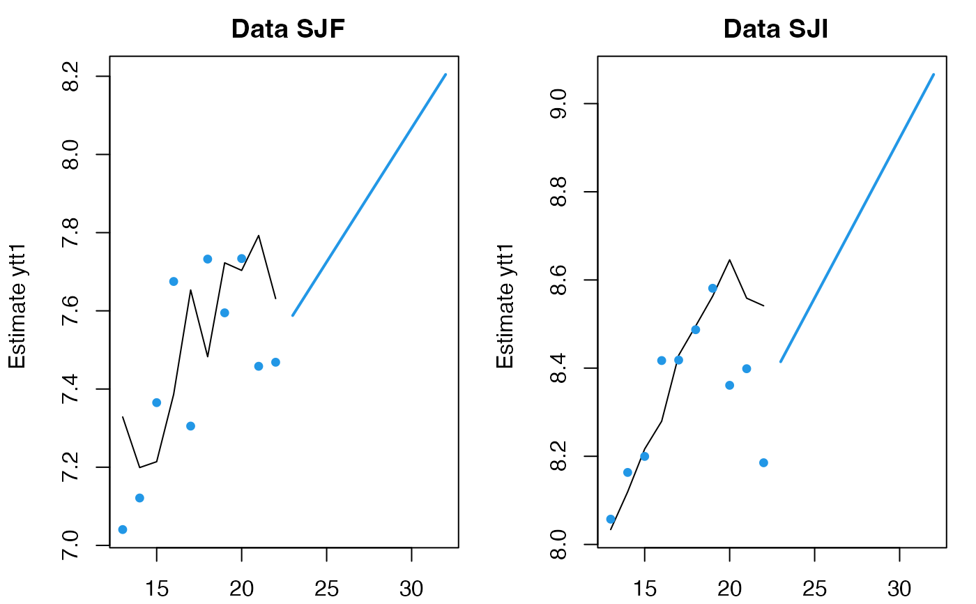
fr <- predict(fit, n.ahead=10)
plot(fr, include=10)


# forecast.marssMLE does the same thing as predict with h
fr <- forecast(fit, n.ahead=10)
plot(fr)


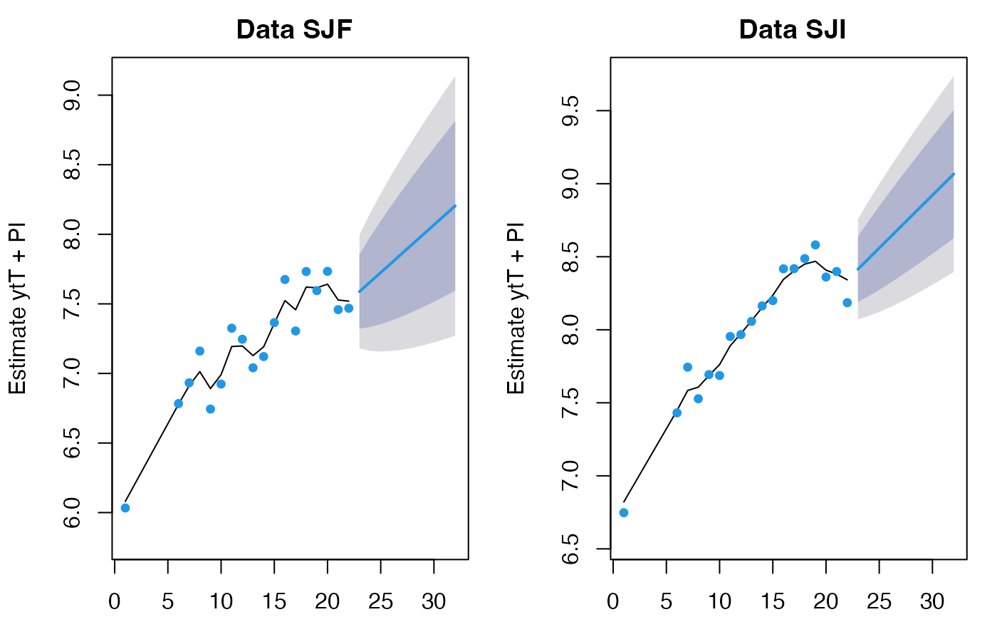# without h, predict will show the prediction intervals
fr <- predict(fit)
plot(fr)


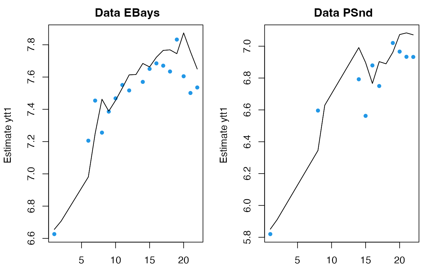
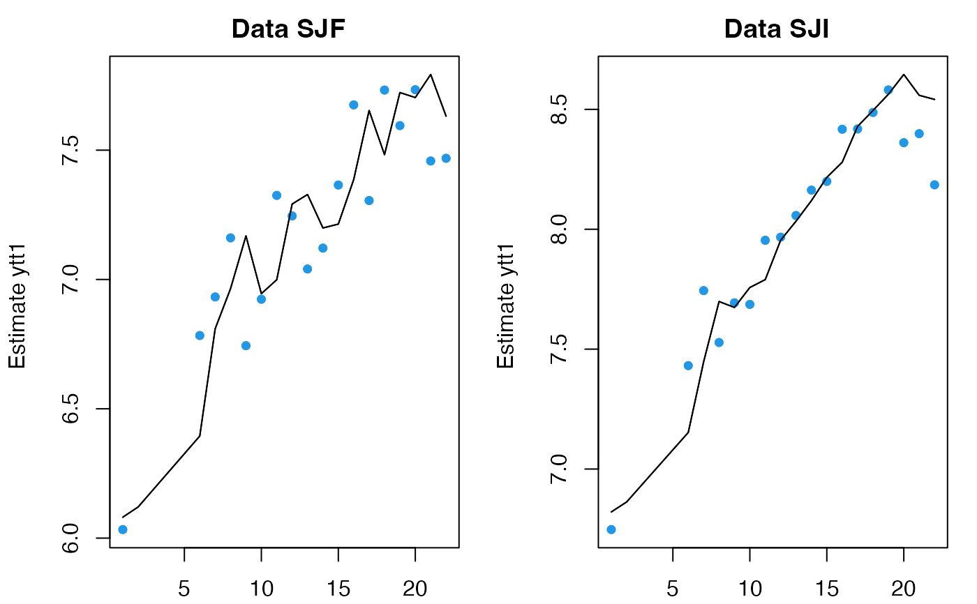# you can fit to a new set of data using the same model and same x0
fr <- predict(fit, newdata=list(y=dat[3:4,]), x0="use.model")
plot(fr)


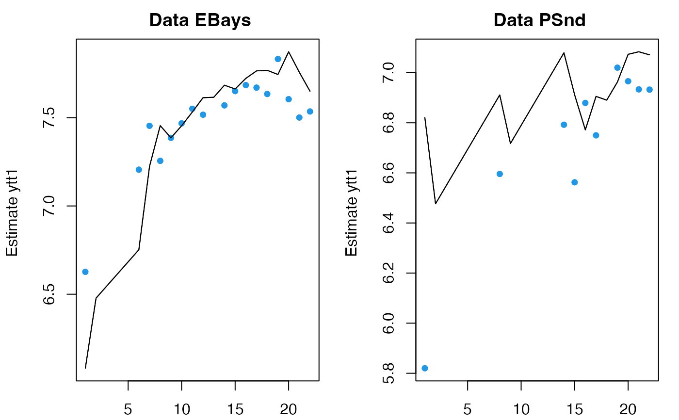# but you probably want to re-estimate x0
fr <- predict(fit, newdata=list(y=dat[3:4,]), x0="reestimate")
plot(fr)


# forecast; note h not n.ahead is used for forecast()
fr <- forecast(fit, h=10)