Plot MARSS MLE objects — plot.marssMLE • MARSS

Plots fitted observations and estimated states with confidence intervals using base R graphics (plot) and ggplot2 (autoplot). Diagnostic plots also shown. By default a subset of standard diagnostic plots are plotted. Individual plots can be plotted by passing in plot.type. If an individual plot is made using autoplot(), the ggplot object is returned which can be further manipulated.

Usage

# S3 method for marssMLE
plot(x, plot.type = c(
    "fitted.ytT", "fitted.ytt", "fitted.ytt1", 
    "ytT", "ytt", "ytt1",
    "fitted.xtT", "fitted.xtt1", 
    "xtT", "xtt", "xtt1",
    "model.resids.ytt1", "qqplot.model.resids.ytt1", "acf.model.resids.ytt1",
    "std.model.resids.ytt1", "qqplot.std.model.resids.ytt1", "acf.std.model.resids.ytt1",
    "model.resids.ytT", "qqplot.model.resids.ytT", "acf.model.resids.ytT",
    "std.model.resids.ytT", "qqplot.std.model.resids.ytT", "acf.std.model.resids.ytT",
    "model.resids.ytt", "qqplot.model.resids.ytt", "acf.model.resids.ytt",
    "std.model.resids.ytt", "qqplot.std.model.resids.ytt", "acf.std.model.resids.ytt",
    "state.resids.xtT", "qqplot.state.resids.xtT", "acf.state.resids.xtT",
    "std.state.resids.xtT", "qqplot.std.state.resids.xtT", "acf.std.state.resids.xtT",
    "residuals", "all"),
    form=c("marxss", "marss", "dfa"),
    standardization = c("Cholesky", "marginal", "Block.Cholesky"),
    conf.int=TRUE, conf.level=0.95, decorate=TRUE, pi.int = FALSE,
    plot.par = list(), ..., silent = FALSE)
# S3 method for marssMLE
autoplot(x, plot.type = c(
    "fitted.ytT", "fitted.ytt", "fitted.ytt1", 
    "ytT", "ytt", "ytt1",
    "fitted.xtT", "fitted.xtt1", 
    "xtT", "xtt", "xtt1",
    "model.resids.ytt1", "qqplot.model.resids.ytt1", "acf.model.resids.ytt1",
    "std.model.resids.ytt1", "qqplot.std.model.resids.ytt1", "acf.std.model.resids.ytt1",
    "model.resids.ytT", "qqplot.model.resids.ytT", "acf.model.resids.ytT",
    "std.model.resids.ytT", "qqplot.std.model.resids.ytT", "acf.std.model.resids.ytT",
    "model.resids.ytt", "qqplot.model.resids.ytt", "acf.model.resids.ytt",
    "std.model.resids.ytt", "qqplot.std.model.resids.ytt", "acf.std.model.resids.ytt",
    "state.resids.xtT", "qqplot.state.resids.xtT", "acf.state.resids.xtT",
    "std.state.resids.xtT", "qqplot.std.state.resids.xtT", "acf.std.state.resids.xtT",
    "residuals", "all"),
    form=c("marxss", "marss", "dfa"),
    standardization = c("Cholesky", "marginal", "Block.Cholesky"),
    conf.int=TRUE, conf.level=0.95, decorate=TRUE, pi.int = FALSE,
    fig.notes = TRUE, plot.par = list(), ..., silent = FALSE)

Arguments

x: A marssMLE object.
plot.type: Type of plot. If not passed in, a subset of the standard plots are drawn. See details for plot types.
standardization: The type of standardization to be used plots, if the user wants to specify a specific standardization. Otherwise Cholesky standardization is used.
form: Optional. Form of the model. This is normally taken from the form attribute of the MLE object (x), but the user can specify a different form.
conf.int: TRUE/FALSE. Whether to include a confidence interval.
pi.int: TRUE/FALSE. Whether to include a prediction interval on the observations plot
conf.level: Confidence level for CIs.
decorate: TRUE/FALSE. Add smoothing lines to residuals plots or qqline to qqplots and add data points plus residuals confidence intervals to states and observations plots.
plot.par: A list of plot parameters to adjust the look of the plots. See details.
fig.notes: Add notes to the bottom of the plots (only for autoplot().
silent: No console interaction or output.
...: Other arguments, not used.

Value

autoplot() will invisibly return the list of ggplot2 plot objects. Use plts <- autoplot() to obtain that list.

Details

The plot types are as follows:

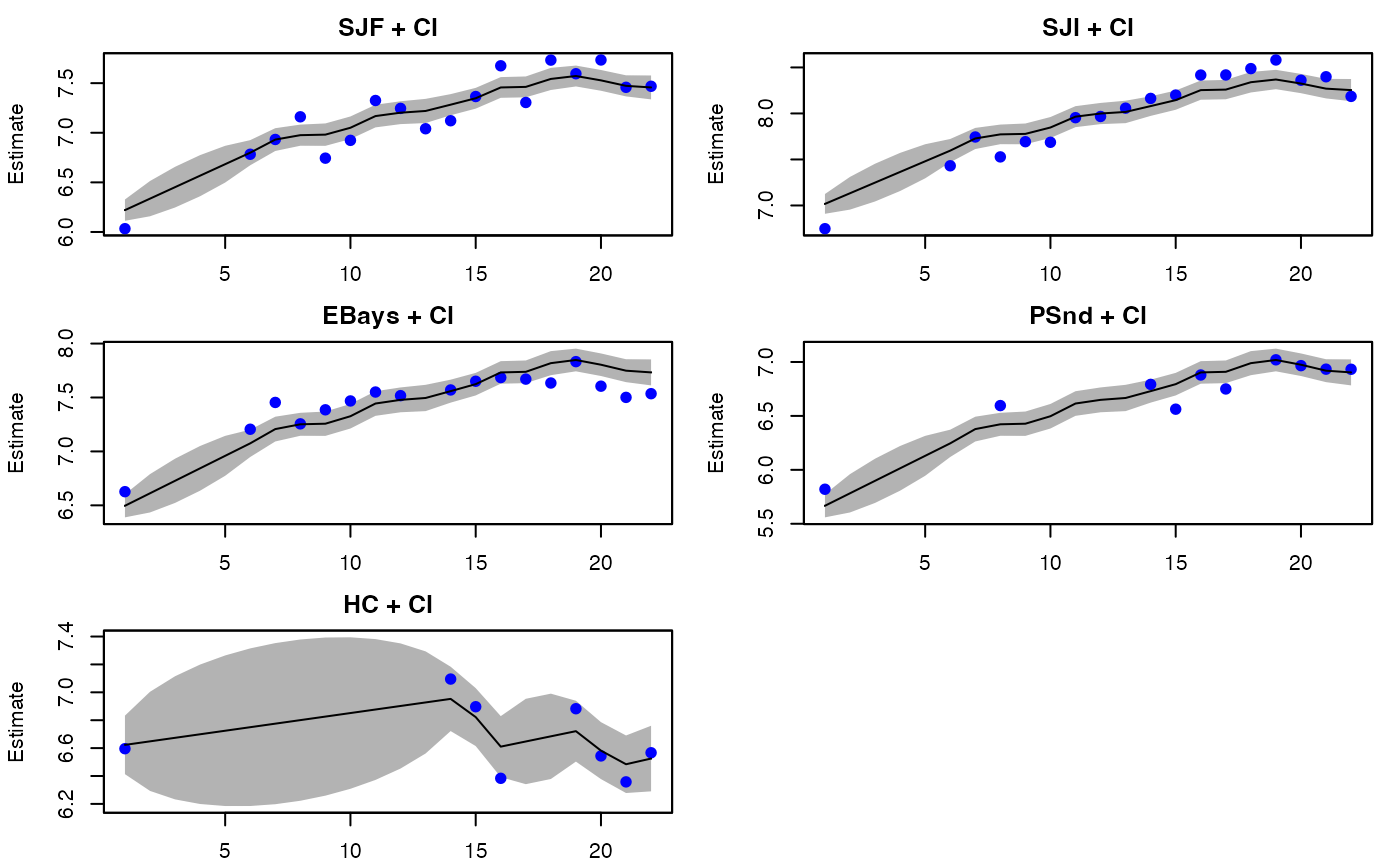
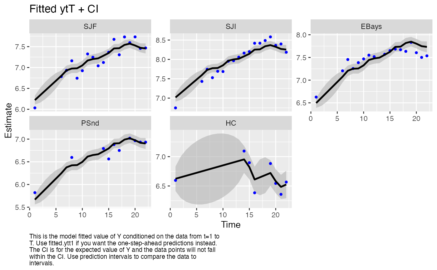
"fitted.y": This plots the fitted \(\mathbf{y}\), which is the expected value of \(\mathbf{Y}\) conditioned on the data from \(t=1\) to \(t-1\), \(t\) or \(T\). It is \(\mathbf{Z}\mathbf{x}_t^T + \mathbf{a}\). The data are plotted for reference but note that the lines and intervals are for new data not the observed data.
"fitted.x": This plots the fitted x, which is the expected value of \(\mathbf{X}\) conditioned on the data from \(t=1\) to \(t-1\) or \(T\). It is \(B \textrm{E}[\mathbf{X}_{t-1}|\mathbf{y}] + u\). The \(\textrm{E}[\mathbf{X}_t|\mathbf{y}]\) are plotted for reference but note that the lines and intervals are for new \(\mathbf{x}\). This is not the estimated states; these are used for residuals calculations. If you want the state estimates use xtT (or xtt).
"xtT": The estimated states from the Kalman smoother (conditioned on all the data).
"xtt1": The estimated states conditioned on the data up to \(t-1\). Kalman filter output.
"model.resids.ytT", "model.resids.ytt1", "model.resids.ytt": Model residuals (data minus fitted y). ytT indicates smoothation residuals, ytt1 indicates innovation residuals (the standard state-space residuals), and ytt are the residuals conditioned on data up to \(t\).
"state.resids.xtT": State smoothation residuals (E(x(t) | xtT(t-1)) minus xtT(t)). The intervals are the CIs for the smoothation residuals not one-step-ahead residuals.
"std": std in front of any of the above plot names indicates that the plots are for the standardized residuals.
"qqplot": Visual normality test for the residuals, model or state.
"acf": ACF of the residuals. The only residuals that should be temporally independent are the innovation residuals: acf.model.residuals.ytt1 and acf.std.model.residuals.ytt1. This ACF is a standard residuals diagnostic for state-space models. The other ACF plots will show temporal dependence and are not used for diagnostics.
"ytT": The expected value of \(\mathbf{Y}\) conditioned on all the data. Use this for estimates of the missing data points. Note for non-missing \(\mathbf{y}\) values, the expected value of \(\mathbf{Y}\) is \(\mathbf{y}\).
"ytt", ytt1: The expected value of \(\mathbf{Y}\) conditioned on the data from 1 to \(t\) or \(t-1\).

The plot parameters can be passed in as a list to change the look of the plots. For plot.marssMLE(), the default is plot.par = list(point.pch = 19, point.col = "blue", point.fill = "blue", point.size = 1, line.col = "black", line.size = 1, line.linetype = "solid", ci.col = "grey70", ci.border = NA, ci.lwd = 1, ci.lty = 1). For autoplot.marssMLE, the default is plot.par = list(point.pch = 19, point.col = "blue", point.fill = "blue", point.size = 1, line.col = "black", line.size = 1, line.linetype = "solid", ci.fill = "grey70", ci.col = "grey70", ci.linetype = "solid", ci.linesize = 0, ci.alpha = 0.6).

Author

Eric Ward and Eli Holmes

Examples

data(harborSealWA)
model.list <- list( Z = as.factor(c(1, 1, 1, 1, 2)), R = "diagonal and equal")
fit <- MARSS(t(harborSealWA[, -1]), model = model.list)
#> Success! abstol and log-log tests passed at 20 iterations.
#> Alert: conv.test.slope.tol is 0.5.
#> Test with smaller values (<0.1) to ensure convergence.
#> 
#> MARSS fit is
#> Estimation method: kem 
#> Convergence test: conv.test.slope.tol = 0.5, abstol = 0.001
#> Estimation converged in 20 iterations. 
#> Log-likelihood: 18.89262 
#> AIC: -17.78524   AICc: -14.11857   
#>  
#>         Estimate
#> A.SJI    0.79679
#> A.EBays  0.27580
#> A.PSnd  -0.55342
#> R.diag   0.02269
#> U.1      0.05889
#> U.2     -0.00466
#> Q.(1,1)  0.00753
#> Q.(2,2)  0.02486
#> x0.1     6.16171
#> x0.2     6.62763
#> Initial states (x0) defined at t=0
#> 
#> Standard errors have not been calculated. 
#> Use MARSSparamCIs to compute CIs and bias estimates.
#> 
plot(fit, plot.type = "fitted.ytT")

#> plot type =  fitted.ytT  Observations with fitted values

require(ggplot2)
autoplot(fit, plot.type = "fitted.ytT")


if (FALSE) {
# DFA example
dfa <- MARSS(t(harborSealWA[, -1]), model = list(m = 2), form = "dfa")
plot(dfa, plot.type = "xtT")
}